Solar Wind Control of the Polar Cusp at High Altitude
1Institute of Geophysics and Planetary Physics, University of California, Los Angeles
2Lockheed Martin, Palo Alto, CA
3University of Iowa, Iowa City, IA
Abstract. The POLAR mission is ideally suited to explore the high-altitude polar cusp. POLAR magnetometer data, together with electron and ion measurements from the HYDRA and TIMAS instruments from March 1996 to December 1997, have been used to identify 459 polar cusp crossings. These crossings are used to study the statistical behavior of the cusp location and its dependence on the solar wind conditions. We find that the invariant latitude of the center of the cusp varies from 70 to 86 degrees as solar wind conditions change and the magnetic local time of the footprints of the cusp magnetic field lines extends from 0800-1600 MLT, the cusp extending slightly further in local time for increasing solar wind dynamic pressure. The average latitude of the center of the cusp is at 80.3o invariant latitude at noon and decreases to 78.7o at 0800 and 1600 MLT. The cusp also appears to thicken slightly in invariant latitude with increasing dynamic pressure. The center of the cusp moves equatorward with increasingly southward IMF to 73o invariant latitude for a 10 nT southward IMF. The cusp moves only slightly for northward IMF. This motion is consistent with erosion of dayside magnetic flux for southward IMF but little or no erosion for northward IMF. The cusp is also somewhat wider in invariant latitude with increasingly northward IMF. Consistent with low altitude observations, we find that there is a clear MLT shift due to the IMF By for strongly southward IMF. We interpret the motion of the local time of the cusp for southward IMF as a shift of the reconnection site away from the noon meridian when the IMF is not due southward.
Introduction
The polar cusp has been studied extensively at low altitudes using observations from the Defense Meteorological Satellite Program (DMSP). With about 5,609 crossings, Newell and Meng [1988] studied the local time dependence of the cusp, showing that it is observed most frequently near magnetic local noon. The effects of dipole tilt angle and the orientation of the interplanetary magnetic field (IMF) on the location of the polar cusp were studied by Newell and Meng [1989] and Newell et al. [1989]. They found that when the IMF is southward, the polar cusp moves equatorward with more negative Bz and when it is northward, the magnetic latitude of the cusp changes very little. When the IMF By component is negative (positive), the cusp shifts dawnward (duskward), while the IMF Bx component has no effect on the cusp position. At high-altitudes our understanding of the cusp behavior is derived mainly from HEOS 2 and Hawkeye observations. Using Hawkeye data in a survey of the polar cusp crossings, Farrell and Van Allen [1990] reported that the latitudinal extent of the cusp region is enlarged when the solar wind dynamic pressure is greater. While these authors reported the same IMF Bz effect on the position of the cusp (see also Zhou and Russell, 1997) as that observed at low altitudes [Newell et al., 1989], a later report by Fung et al. [1997] did not find any significant IMF By effect at high altitudes. Fung et al. [1997] also reported that when solar wind dynamic pressure is greater, the extent in magnetic local time of the polar cusp at high altitudes is smaller.
The POLAR spacecraft provides us an excellent opportunity to study the polar cusp at high altitudes. We identify entries into the polar cusp along the POLAR trajectories with the POLAR magnetic field data [Russell et al., 1995] together with HYDRA [Scudder et al, 1995] and TIMAS [Shelley et al, 1995] key parameter data. The cusp entries occur at altitudes of 4.8 to 8.8 RE in the northern hemisphere. We have reported the location of the cusp and its dependence on the dipole tilt angle in an earlier paper [Zhou et al., 1999]. In this paper we discuss how the local time and invariant latitude of the cusp depends on solar wind dynamic pressure, and IMF By and Bz.
Examples of Cusp Crossings
In the cusp region, we expect to see magnetosheath-like (high density and low energy) plasma. Further at high altitudes, the plasma causes a diamagnetic depression and fluctuations in the magnetic strength, because the plasma in the polar cusp region has an energy density that is significant relative to background magnetic field in contrast to low altitudes where the magnetic energy density is far greater than that of the plasma. As described in our previous paper [Zhou et al., 1999] the criteria used to identify the cusp crossings are: fluctuations in the magnetic field; a greater than 1 nT depression of the magnetic field strength below the neighboring background level; a sudden increase in the low-energy ion and electron density that is greater than 5 cm-3; electron thermal energy less than 100 eV; and the presence of significant He++, which indicates solar wind origin for the plasma.
The four panels of Figure 1 show examples of polar cusp crossings for northward, southward, eastward and westward IMF. The upper trace in each panel shows the residual of the magnitude of POLAR MFE data with the Tsyganenko 96 model [Tsyganenko and Stern, 1996]. The second and third traces show the Hydra electron density and energy. The fourth and fifth traces show the Timas low energy range H+ density and temperature. Not shown is the He++ density. The vertical dashed lines indicate the polar cusp entry and exit.
In the upper left panel of Figure 1, the polar cusp is found from 0457-0532 UT, corresponding to a magnetic local time of the footprint on the surface of the Earth 1214-1250 MLT. During this period POLAR moves from (3.05, -0.09, 5.91) RE to (2.70, 0.30, 6.64) RE in SM coordinates. The residual between the MFE data and Tsyganenko 96 model is about 20 nT, the highest electron density is 28 cm-3, the electron energy is about 40 eV. The data from the Timas low energy range H+ shows that the density is 13 cm-3, and the energy is 90 eV. These are all consistent with the criteria discussed above. In this case, the solar wind dynamic pressure is 2.3 nPa, IMF By=-0.6 nT, Bz=2.3 nT. The solar wind conditions are derived from the WIND key parameters and are time-shifted according to the distance along the Earth-sun line from the WIND spacecraft to 10 RE and the solar wind velocity Vx component in GSM. The invariant latitude ranges from 79.7°-81.9°. The invariant latitude, here and throughout the paper, was determined by field-line tracing the Tsyganenko 96 model for a dynamic pressure of 2 nPa. The results of this study are not sensitive to this choice of pressure.
The upper right panel shows an example of southward IMF conditions. The solar wind has a dynamic pressure of 2.8 nPa; an IMF By of -5.5, and Bz of -9.7 nT. The POLAR spacecraft is in the cusp from 1740-1750 UT at a magnetic local time from 1116 to 1114 MLT. The magnetic local time was obtained from the difference in magnetic longitude of the northern cusp foot point and that of the subsolar point. As it transverses the cusp plasma POLAR moves from (3.42, -0.39, 3.87) RE to (3.37,-0.41, 4.19) RE. This case has one of the largest southward Bz values in our entire data set. The invariant latitude ranges from 73.0-74.2o. This is also a low invariant latitude for the cusp, but it is not the lowest in the data set.
The lower left panel shows a case for eastward IMF. The solar wind conditions are: a dynamic pressure of 3 nPa; an IMF By component of 4 nT, and a Bz component close to 0 nT. The position ranges from (2.81, 0.24, 5.77) RE to (2.40, 0.79, 6.61) RE in SM. The magnetic local time is 1317-1410 MLT, so that the entire pass took place postnoon.
The lower right panel is an example of westward IMF. The solar wind conditions are: dynamic pressure
1.6 nPa; IMF By=-4.2, and Bz= -0.1 nT. The position ranges from (2.33, -0.53, 6.33) RE to (2.71, -0.44, 5.41)
RE in SM. The magnetic local time ranges from 1018 to 1056 MLT.
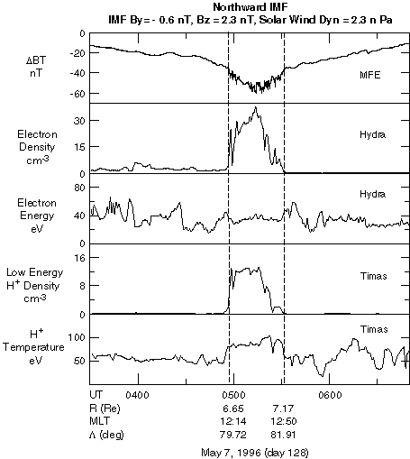
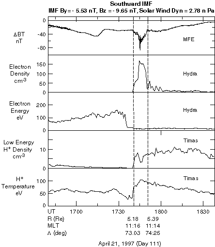
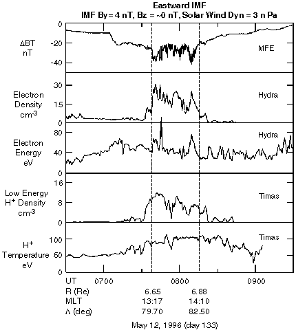
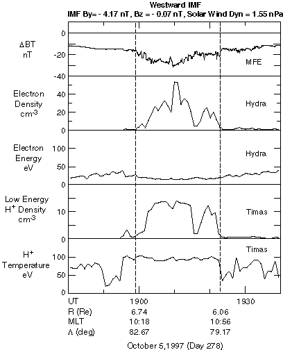
Figure 1. Examples of polar cusp crossings for (top left) northward,
(top right)
southward, (lower left) eastward and (lower right) westward IMF respectively. The upper trace shows the residual of the
magnitude of POLAR MFE data with Tsyganenko 96 model. The second and third traces show the Hydra electron density and
energy. The fourth and fifth traces show the Timas H+ density and temperature in the energy range 15 eV to
370 eV. The vertical dashed lines indicate the polar cusp crossings.
The Polar Cusp Location
Figure 2 shows the local time and invariant latitude distribution of the footprints of the cusp boundaries, calculated using the Tsyganenko 96 model to trace the magnetic field lines down to the surface of the Earth. The left panel shows the equatorward boundary of the cusp, while the right panel shows the poleward boundary. We remove the dipole tilt-angle effect from these plots based on the observation that the invariant latitude of the cusp increases 1 degree for every 14 degrees increase in the tilt angle [Zhou et al., 1999]. We also restrict these plots in which the solar wind dynamics pressure was less than 4 nPa, to avoid the mantle region and broad cusp observed near the magnetopause. The polar cusp is located from 69° to 87° invariant latitude and the magnetic local time of these crossing ranges from about 0700-1700 MLT. The large scatter is due principally to the motion of the cusp caused by the variations in the IMF that we discuss below.
The central horizontal bars in the figures show the median values. At noon the median upper border of
the cusp is 81.5o and the lower border is 78.8o invariant latitude. The smooth curves show the
least square fit to the median positions as a function of local time. We use the following function to fit the data.
The parameters (![]() 0 and A) are shown in Table 1.
0 and A) are shown in Table 1.
| (1) |
where Table 1. The Least Square Fit to the Polar Cusp Position
![]() is the invariant latitude, MLT is the magnetic local time in
hours. Also shown in the table are the standard deviation of the residuals of the fit to the 8 median values, and the
correlation coefficient.
is the invariant latitude, MLT is the magnetic local time in
hours. Also shown in the table are the standard deviation of the residuals of the fit to the 8 median values, and the
correlation coefficient.
|
|
|
A |
|
R |
|
Equatorward Boundary |
78.8° |
0.11 |
0.73 |
0.83 |
|
Poleward Boundary |
81.8° |
0.095 |
0.04 |
0.94 |
 2
2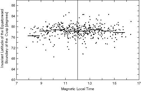 |
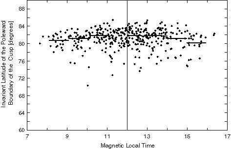 |
| Figure 2. The invariant latitude-magnetic local time distribution of the polar cusp boundaries: (left) the equatorward boundary; (right) the poleward boundary. The central horizontal bars in the figures show the medians every hour of magnetic local time. | |
The Solar Wind Control
There is much scatter in Figure 2. Since dipole tilt effects [Zhou et al., 1998] have been removed in this study, the scatter here is due to the solar wind conditions. The cusp changes with solar wind dynamic pressure, IMF Bz and IMF By. Figure 3 shows the invariant latitude of the center of cusp crossings versus IMF Bz again restricted to solar wind dynamic pressures of less than 4 nPa. The cusp center is taken as the average of the entry and exit locations in latitude and longitude. We note that the cusp at the altitude of Polar is long (in local time) and narrow (in latitude) and does not appear to thin with distance from noon. This geometry together with the near vertical line of upsides of the Polar spacecraft means that there are no grazing encounters with the cusp. The spacecraft generally penetrated the cusp cleanly. The horizontal bars indicate the median invariant latitudes within different IMF Bz ranges. For IMF Bz<0, when IMF is more negative, the cusp moves more equatorward, but when IMF Bz>0 the cusp latitude is approximately constant.
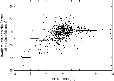 |
Figure 3. The invariant latitude of the center of cusp versus IMF Bz. The horizontal bars indicate the median invariant latitudes every 2 nT of IMF BZ GSM. |
In Table 2, we show the parameters of the least square fit to the medians shown in Figure 3 to the equation:
| (2) |
Table 2. Least Square Fit to the Latitude of the Cusp as a Function of the IMF
North-South Component
|
Cusp Parameter |
IMF Bz |
|
m |
|
R |
|
Center |
N |
80.7° |
-0.027 |
0.02 |
0.53 |
|
Center |
S |
81.3° |
0.98 |
0.41 |
0.98 |
|
Equatorward Edge |
N |
79.2° |
-0.07 |
0.03 |
0.76 |
|
Equatorward Edge |
S |
79.5° |
0.86 |
0.22 |
0.99 |
|
Poleward Edge |
N |
82.0° |
0.02 |
0.02 |
0.35 |
|
Poleward Edge |
S |
83.0° |
1.08 |
0.78 |
0.97 |
|
Cusp Width |
N & S |
2.75° |
0.09 |
0.22 |
0.75 |
For southward IMF, the invariant latitude of the center of the cusp in degrees becomes just under 1° further equatorward for every 1 nT of southward IMF. The correlation coefficient of the fit is 98%. For northward IMF, the slope is slightly negative (-0.027), i.e., the cusp moves slightly equatorward for increasingly northward IMF. According to the standard t-test, the correlation coefficient of 53% indicates that the slope is inconsistent with the null hypothesis at the 86% level.
The variations of the equatorward and the poleward boundaries with IMF Bz are shown in Figure 4. The fits to the medians are also given in Table 2 for both cases. The two boundaries behave the same way as the center of the cusp. The boundaries move equatorward for southward IMF but remain nearly fixed for northward IMF. The equatorward boundary moves 0.86° equatorward for each nT of southward IMF and 0.07° equatorward for each nT of northward field. The latter variation has a correlation coefficient of 0.76 and is inconsistent with the null hypothesis at the 98% level. The poleward edge moves equatorward 1.08° for every 1 nT of southward field and moves 0.02° for every 1 nT of northward IMF. This latter variation is inconsistent with the null hypothesis at the 74% level.
We have used our best estimate for the instantaneous magnetic field in the solar wind near the Earth using WIND data time-shifted by the solar wind convection time in the x direction. This is consistent with the near immediate response of the location of the cusp to IMF By changes found by Moen et al. [1999]. However, the cusp lies roughly at the boundary between the dayside magnetic field lines and those that are swept into the tail and this interface moves as magnetic flux is carried from the dayside into the tail. Since the location of the cusp should be related both to the history of the IMF and of reconnection in the tail, we do not expect the polar cusp to immediately move to its new equilibrium position in response to a change in the IMF direction and there will be some scatter in this result. To take the effect into account in the motion of the cusp would require both a study of the time history of the IMF and the time since the last substorm in the tail. Since this would be a daunting task in a statistical study of this size, we defer it at this time.
As in our study of the invariant latitude of the cusp with local time, we find from the coefficients
in Table 2 that the cusp is about 3o wide in the latitudinal direction, varying slightly with the north-south
component of the IMF.
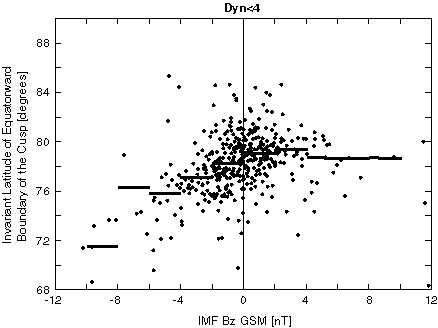
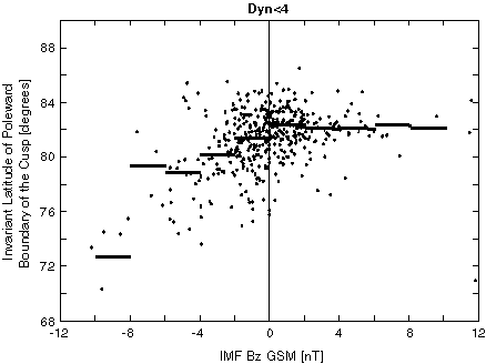
Figure 4. The invariant latitude of (left) the equatorward boundary,
(right) the poleward
boundary of the cusp versus IMF Bz. The horizontal bars indicate the median invariant latitudes every 2nT of Bz.
We show explicitly the latitudinal width of the cusp as a function of IMF Bz observed on individual passes in Figure 5. The least squares fit to the medians given in Table 2 indicates that the cusp increases in width with increasingly northward IMF Bz. The cusp is about 2o wide for an IMF Bz of -10 nT and 4o wide for an IMF Bz of 10 nT.
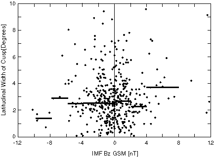 |
Figure 5. The width of the cusp in invariant latitude versus IMF Bz. Horizontal bars show the median values of the width every 2 nT in Bz. |
We now consider the effect of IMF By on the cusp position. Figure 6 shows the local time of the
encounter with the center of the cusp versus the IMF By for each of three ranges of IMF Bz, northward, horizontal and
southward. The northward fields are defined as those more than 15o above the horizontal direction in GSM
coordinates and the southward fields are defined as those more than 15o below the horizontal. Periods of
dynamic pressure greater than 4 nPa have been omitted from these panels. The short vertical bars indicate the medians of
the magnetic local time within each 2 nT increment of IMF By. For positive IMF By and northward IMF, there is one bar in
the prenoon sector, and three in the postnoon sector. For negative IMF By, there are one in the prenoon and two in the
postnoon sector. This is not a significant variation with By.
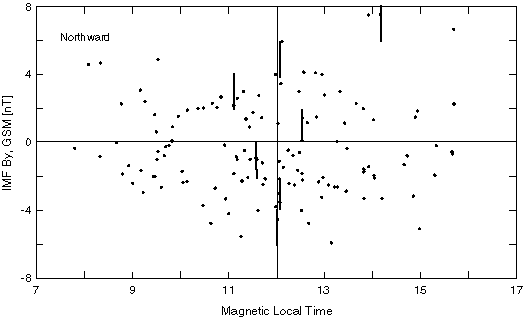
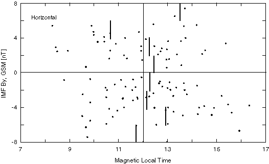
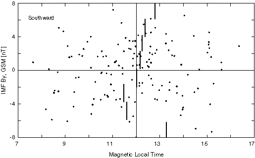
Figure 6. The local time of the center of the cusp crossings versus the IMF By: (upper) for
northward IMF;(center) for horizontal and (lower) for southward IMF. Vertical bars show median values of the magnetic
local time every 2 nT of By.
For horizontal IMF, there are one prenoon and three postnoon for positive By and one prenoon and three postnoon for negative By. Again this is not a significant variation althougth there is a tendency to change local time with changing By in the direction found by Newell et al [1989]. For southward IMF, there is clearly a duskward (dawnward) shift for positive (negative) IMF By. Only one point, and one with poor statistics, seems to not follow this trend. This shift is in the same direction as seen at low altitudes in the northern hemisphere. We recall that all the data studied here were obtained in the northern hemisphere, while the low altitude data were obtained in both hemispheres.
In Table 3 we show the parameters of the least square fit to the medians shown in Figure 7 to the equation:
| MLT = MLT0 + b*IMF By | (3) |
Table 3. Parameters for the Least Square Fit to the IMF By Effect
|
|
MLT0 |
b |
|
R |
|
Bz Northward |
12.12 |
0.106 |
0.72 |
0.47 |
|
Bz Horizontal |
12.25 |
0.009 |
0.69 |
0.05 |
|
Bz Southward |
11.83 |
0.103 |
0.02 |
0.96 |
Next, we investigate the possible effects of the solar wind dynamic pressure on the dimensions of the polar cusp. Figure 7 illustrates the relation between the solar wind dynamic pressure and the width in invariant latitude of the polar cusp crossings. The bars show the median values of the latitudinal width. An upward trend in the width with greater solar wind dynamic pressure is seen. Since the spacecraft is closer to the magnetopause when the dynamic pressure is greater this result may just reflect the geometry of the cusp near the magnetopause. Thus in earlier studies in this paper we have restricted our statistics to periods when the dynamic pressure was less than 4 nPa.
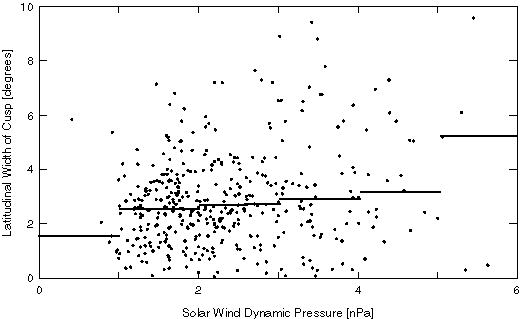 |
Figure 7. The relation between the solar wind dynamic pressure and the latitudinal width of the polar cusp crossings. Horizontal bars show the medians over intervals of 1 nPa. |
Finally, there is also a correlation between the solar wind dynamic pressure and the polar cusp extent in magnetic local time. This correlation is shown in Figure 8 in which the solar wind dynamic pressure at each cusp crossing is plotted versus the location of the center of the polar cusp in magnetic local time. The bars are medians for different magnetic local time ranges calculated using the full widths of the local time of each cusp crossing. Since the solar wind dynamic pressure is independent of the location of the Polar spacecraft, the rise in solar wind dynamic pressure at the edges of this plot indicates that the cusp extends further away from local noon when the solar wind dynamic pressure is stronger.
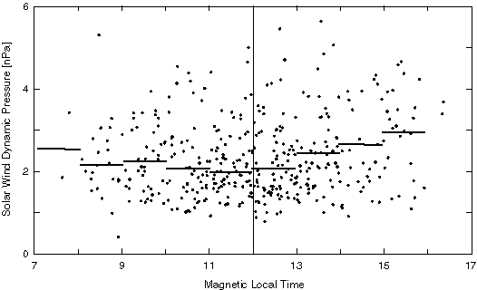 |
Figure 8. The magnetic local time of the center of the polar cusp crossings versus solar wind dynamic pressure. Horizontal bars show median solar wind pressure for each hour of MLT. |
Discussion and Conclusions
The polar cusp crossings we have shown here occur at a radial distance of 5-9 RE which is well above the location of the DMSP observations upon which much of our understanding of the polar cusp is based and below those of HEOS and Hawkeye. This provides us a good opportunity to compare the behavior of the low-altitude cusp with its high-altitude counterpart. The properties of the cusp that we have found in our survey of the POLAR data confirm many of the previous results but also show some apparent discrepancies and provide some new insights. These earlier results can be found in papers covering the low-altitude observations by DMSP satellites [Newell and Meng, 1987; 1988; 1989; Newell et al., 1989] and the high-altitude observations by Hawkeye [Farrell and Van Allen, 1990; Zhou and Russell, 1997; Fung et al., 1997].
Since the cusp region is "open" to the solar wind, we expect its properties to be intimately controlled by it. The low-altitude observations show both the IMF Bz and IMF By effects on the polar cusp position, while the Hawkeye observations show the IMF Bz effect [Zhou and Russell, 1997] but not the IMF By effect [Fung et al., 1997]. In this paper, we have demonstrated that when the IMF is more southward the center of the cusp moves equatorward, which is consistent with the previous results and our present understanding of the IMF effects on the magnetosphere. This motion can be interpreted in terms of the erosion of the magnetopause [Aubry et al., 1970] in which southward IMF carries magnetic flux from the dayside closed field lines into the open tail. The cusp that exists on the newly opened field lines moves equatorward as the flux content of the tail increases. When a substorm occurs, this flux is returned to the dayside magnetosphere and the cusp will move poleward [Russell and McPherron, 1973]. The slope of dependence on the IMF seen at both low and high altitudes is very similar but the low altitude observations of the cusp lie about 1.5 degrees equatorward of the high altitude observations. We attribute the difference to the use of hourly average IMF in the low altitude study in contrast to the one minute average used here. Since the cusp position depends in part on an integral of the history of the IMF Bz we expect the long term average will give a more equatorward or eroded position. Regarding the IMF Bz effect on the cusp width, Newell and Meng [1987] reported that the cusp narrows following a southward turning of the IMF Bz. We also find a slight narrowing as the IMF becomes increasingly southward, and some thickening for northward IMF. In particular the equatorward boundary moves slightly further equatorward with increasingly northward IMF.
We also see a very clear local time shift due to different IMF By when the IMF is southward. Upon reconnection with southward IMF, the newly opened northern hemisphere magnetic flux will be dragged by positive IMF By toward the dawnside, but the cusp is seen to move toward the afternoon side in this hemisphere. In contrast Newell at al. [1989] also see a cusp displacement in the northern hemisphere toward the afternoon under these conditions. Newell et al. [1989] interpreted this result in terms of the expected displacement of reconnection sites away from noon when the IMF is not due southward [Crooker, 1979; Luhmann et al., 1984]. For positive By the center of the reconnection site moves duskward in the northern hemisphere and dawnward in the southern hemisphere. Since each reconnection site is connected to both the northern and southern hemispheres, this mechanism might be expected to split the cusp and move the two parts away from noon. However, in MHD simulations this is not what happens. Rather the reconnection site affects most the ionosphere to which it is closest [Russell et al., 1999]. At Polar altitudes (for a dynamic pressure of less than 4 nPa) the southward control of the cusp position is found to be consistent with the low altitude results. When the IMF is northward the effect is weaker at low altitudes [Newell et al. 1989] and statistically insignificant in the POLAR data. It is possible that the difference between the high altitude and low altitude studies here is again due to the different averaging periods used for the IMF data.
Regarding the effects of solar wind dynamic pressure on the polar cusp locations, we see that it thickens the cusp in the latitudinal direction and also widens the extent in magnetic local time, the longitudinal direction. The former result is consistent with that reported by Farrell and Van Allen [1990] using the Hawkeye data. However, the latter result appears to be at odds with that reported by Fung et al. [1997], also based on Hawkeye observations, that higher solar wind dynamic pressure shrinks the cusp extent in magnetic local time.
In conclusion, we have identified 459 polar cusp crossings from the POLAR magnetic field data along with the HYDRA and TIMAS key parameter data from March 1996 to December 1997. Statistically, the cusp can be usually found from 0800-1600 MLT. The invariant latitude of the center of the cusp extends from 70° to 86° degrees and moves further equatorward for stronger southward IMF. We clearly see a local time shift due to the IMF By only for southward IMF conditions. The higher solar wind dynamic pressure widens the cusp region in the latitudinal direction and extends it in the longitudinal direction.
Acknowledgements
This research was supported by the National Aeronautics and Space Administration at UCLA under research grant NAG5-3171; at Lockheed Martin under contract NAS5-30302; and at the University of Iowa under grant NAG5-2231.
References
Aubry, M.P., C.T. Russell, and M.G. Kivelson, Inward motion of the magnetopause before a substorm, J. Geophys. Res., 75, 7018-7031, 1970.
Crooker, N. U., Dayside merging and cusp geometry, J. Geophys. Res., 84, 951-959, 1979.
Farrell, W. M., and J. A. Van Allen, Observations of the Earth's polar cleft at large radial distances with the Hawkeye 1 magnetometer, J. Geophys. Res., 95, 20945-20958, 1990.
Fung, S. F., T. E. Eastman, S. A. Boardsen and S.-H. Chen, High-Altitude Cusp Positions Sampled by the Hawkeye Satellite, Physics and Chemistry of the Earth, 22, 653-662, 1997
Luhmann, J. G., R. J. Walker, C. T. Russell, N. U. Crooker, J. R. Spreiter and S. S. Stahara, Patterns of potential magnetic field merging sites on the dayside magnetopause, J. Geophys. Res., 89, 1739-1742, 1984.
Moen, J., H. C. Carlson and P. E. Sandholt, Continuous observation of cusp auroral dynamics in response to an IMF By polarity change, Geophys. Res. Lett., 26, 1243-1246, 1999
Newell, P. T. and C.-I. Meng, Cusp width and Bz: observations and a conceptual model, J. Geophys. Res., 92, 13673-13678, 1987.
Newell, P. T. and C.-I. Meng, The cusp and cleft/boundary layer: Low altitude identification and statistical local time variation, J. Geophys. Res., 93, 14549-14556, 1988.
Newell, P. T. and C.-I. Meng, Dipole tilt angle effects on the latitude of the cusp and cleft/low-latitude boundary layer, J. Geophys. Res., 94, 6949-6953, 1989.
Newell, P. T., C.-I. Meng, D. G. Sibeck, and R. P. Lepping, Some low-altitude cusp dependencies on interplanetary magnetic field, J. Geophys. Res., 94, 8921-8927, 1989.
Russell, C. T., The polar cusp, Adv. Space Res., in press, 1999
Russell, C. T. and R. L. McPherron, The semiannual variation of geomagnetic activity, J. Geophys. Res., 78(16), 3068, 1973
Russell, C. T., R. C. Snare, J. D. Means, D. Pierce, D. Dearborn, M. Larson, G. Barr and G. Le, The GGS POLAR magnetic fields investigation, Space Sci. Rev., 71, 563-582, 1995.
Scudder, J., F. Hunsacker, G. Miller, J. Lobell, and others, HYDRA - a 3-dimensional electron and ion hot plasma instrument for the POLAR spacecraft of the GGS mission, Space Sci. Rev., 71, 459-495, 1995.
Shelley, E.G., A. G. Ghielmetti, H. Balsiger, R. K. Black, and others, The Toroidal Imaging Mass-Angle Spectrograph (TIMAS) for the POLAR mission, Space Sci. Rev., 71, 497-530, 1995
Tsyganenko, N. A., and D. P. Stern, Modeling the global magnetic field of the large-scale Birkeland current systems, J. Geophys. Res., 101, 27187-27198, 1996
Zhou, X.-W. and C. T. Russell, The location of the high-latitude polar cusp and the shape of the surrounding magnetopause, J. Geophys. Res., 102, 105-110, 1997
Zhou, X. W., C. T. Russell, G. Le, S. A. Fuselier and J. D. Scudder, The polar cusp location and its dependence on dipole tilt, Geophys. Res. Lett., 26, 429-432, 1999.
 Back to CT Russell's page
 More On-line Resources
Back to the SSC Home Page
More On-line Resources
Back to the SSC Home Page