MAGNETOPAUSE LOCATION UNDER EXTREME
SOLAR WIND CONDITIONS
J.-H. Shue1, P. Song2, C. T. Russell3,
J. T. Steinberg4, J. K. Chao5, G. Zastenker6,
O. L. Vaisberg6, and S. Kokubun1, H. J. Singer7,
T. R. Detman7, and H. Kawano1,8
1Solar-Terrestrial Environment Laboratory, Nagoya University,
Toyokawa, Japan
(Now at Applied Physics Laboratory, The Johns Hopkins University,
Laurel, Maryland)
2 Space Physics Research Laboratory, The University of
Michigan, Ann Arbor, MI, USA
3Institute of Geophysics Planetary Physics, University
of California, Los Angeles, LA, USA
4Center for Space Research, Massachusetts Institute of
Technology, Cambridge, MA, USA
5Institute of Space Science, National Central University,
Chungli, Taiwan
6Space Research Institute, Russian Academy of Sciences,
Moscow , Russia
7National Oceanic and Atmospheric Administration, Space
Environment Center, Boulder, CO, USA
8Now at Department of Earth and Planetary Sciences, Kyushu
University, Hakozaki, Fukuoka, Japan
Originally published in: J. Geophys. Res., 103, 17,691-17,700, 1998.
Abstract. During the solar wind dynamic pressure enhancement, around 0200 UT on
January 11, 1997, at the end of the January 6-11 magnetic cloud event,
the magnetopause was pushed inside geosynchronous orbit. The LANL 1994-084
and GMS 4 geosynchronous satellites crossed the magnetopause and moved
into the magnetosheath. Also, the Geotail satellite was in the magnetosheath
while the Interball 1 satellite observed magnetopause crossings. This event
provides an excellent opportunity to test and validate the prediction capabilities
and accuracy of existing models of the magnetopause location for producing
space weather forecasts. In this paper, we compare predictions of
two models: the Petrinec and Russell [1996] model and the Shue
et al. [1997] model. These two models correctly predict the magnetopause
crossings on the dayside; however, there are some differences in
the predictions along the flank. The Shue et al. [1997] model
correctly predicts the Geotail magnetopause crossings and partially predicts
the Interball 1 crossings. The Petrinec and Russell [1996] model
correctly predicts the Interball 1 crossings and is partially consistent
with the Geotail observations. We further found that some of the inaccuracy
in Shue et al.'s predictions is due to the inappropriate linear extrapolation
from the parameter range for average solar wind conditions to that for
extreme conditions. To improve predictions under extreme solar wind
conditions, we introduce a nonlinear dependence of the parameters on the
solar wind conditions to represent the saturation effects of the solar
wind dynamic pressure on the flaring of the magnetopause and saturation
effects of the interplanetary magnetic field Bz on the
subsolar standoff distance. These changes lead to a better agreement with
the Interball 1 observations for this event.
1. Introduction
The location of the magnetopause is one of the most important parameters
in space physics because it is the boundary that separates the magnetospheric
plasma from the solar wind and determines the size of the magnetosphere.
Chapman and Ferraro [1931] first introduced the concept of the magnetopause
location which depends on the solar wind dynamic pressure (Dp).
Ferraro [1952] first calculated the size of the magnetosphere
and the shape of the magnetopause. Over the past few decades, space physicists
have exerted much effort to model the location of the magnetopause under
various solar wind conditions. In most of the early work, the location
of the magnetopause depends solely on the solar wind dynamic pressure.
Subsequently, Aubry et al. [1970] first recognized that the interplanetary
magnetic field (IMF) orientation can also affect the magnetopause location.
Later, more empirical models of the magnetopause location were developed
using large in situ data sets of magnetopause crossings [Howe and Binsack,
1972; Formisano et al., 1979; Sibeck et al., 1991; Petrinec
et al., 1991; Petrinec and Russell, 1993, 1996; Roelof and
Sibeck, 1993; Shue et al., 1997]. Some of models [Fairfield,
1971; Howe and Binsack, 1972; Formisano et al., 1979; Petrinec
et al., 1991; Sibeck et al., 1991] define the magnetopause size
and shape for each parameter range but are not valid for the broad, and
especially extreme, ranges of solar wind conditions. The most recent
empirical models [Roelof and Sibeck, 1993; Petrinec and Russell
1996; Shue et al., 1997] provide mathematical expressions for
the size and shape of the magnetopause as functions of the north-south
component of the IMF and the solar wind dynamic pressure. An important
consequence emerging from these new models is that the magnetopause becomes
predictable for any given upstream conditions. In this study, we
compare predictions from the Petrinec and Russell [1996] model and
the Shue et al. [1997] model with in situ observations for
a particular event. We are not comparing with the Roelof and Sibeck
[1993] model because our test conditions are outside the stated range of
validity of the model.
These two models assume cylindric symmetry around the aberrated Sun-Earth
line and have been derived with data sets that are for normal, rather than
extreme, solar wind conditions. Both Shue et al. [1997] and
Petrinec and Russell [1996] claim their models are valid over a
wide solar wind parameter range. The detailed information about the databases
and methods used to derive the two models will be discussed in section
2.
A magnetic cloud arrived at Earth on January 10-11, 1997. During
this event, at 1115 UT on January 11, there was a failure of a geosynchronous
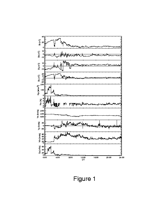
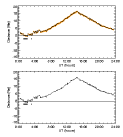
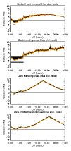
communication satellite (Telstar 401). Also, as shown in Figure
1, during this event, around 0200 UT on January 11, while the interplanetary
magnetic field was extremely strong and northward (~18 nT), there was a
sudden enhancement in the solar wind dynamic pressure up to 60 nPa (including
the contribution from helium ions). The magnetopause was pushed inside
geosynchronous orbit because of the strong compression during this pressure
enhancement which was 30 times more than the average solar wind dynamic
pressure. Many satellites (LANL 1994-084, GMS 4, Geotail, and Interball
1) observed magnetopause crossings during this interval. Thus this
event provides an excellent opportunity to test and validate the prediction
capabilities and accuracy of existing empirical models of the magnetopause
location for both space weather purposes and improving our scientific
understanding. As will be shown in section 3, the two models provide
similar magnetopause locations on the dayside; however, the predictions
on the nightside are different under extreme solar wind conditions.
| Figure 1. Magnetic field (B) and
plasma data from the WIND satellite on January 11, 1997, in GSM coordinates.
The solar wind dynamic pressure (Dp) includes the helium
contribution by a factor (1+0.04Nalpha), where Nalpha
is the He++ concentration (an average value of 4% is used when Nalpha
is missing). The Vth is the thermal speed of the solar wind. |
2. Summary and Comparison of the Two Models
From a mathematical point of view, the models developed by Shue et
al. [1997] and Petrinec and Russell [1996] were derived from
best fits to observed magnetopause locations. The major differences are
the databases, the functional form of the magnetopause, and the specific
dependence of the magnetopause
on the upstream solar wind.
2.1. Shue et al. [1997] Model
On the basis of a database of crossings from ISEE 1 and 2, AMPTE/IRM,
and IMP 8 satellites, the locations of the magnetopause were fit to the
functional form
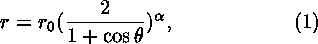
where r is the radial distance and theta is the solar
zenith angle. The positions Xs and Rs
(subscript s denotes the Shue et al. [1997] model) are calculated
by Xs = r * cos(theta) and Rs
= r * sin(theta). This form has two parameters, r0 and
alpha, representing the standoff distance at the subsolar point
and the level of tail flaring, respectively. A very important feature
of this functional form is that the tail magnetopause can be either open
(r goes to infinity when theta = pi) or closed (r
approaches a finite value when theta = pi), depending on the value
of alpha. Almost all other models used an elliptic equation as the
basic functional form. Since an ellipse must close at some point
on the nightside, it cannot represent the magnetopause for an open magnetosphere
[Fairfield, 1995]. Both r0 and alpha depend
on the IMF Bz (in nanoteslas) and the solar wind dynamic
pressure Dp (in nanopascals). Using a bivariant best
fit, Shue et al. [1997] obtained
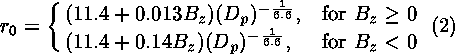

From these relations, the dependence of r0 on the IMF Bz
changes at Bz = 0 nT. A greater slope for the southward
IMF reflects the erosion of the magnetopause associated with dayside reconnection.
More magnetic flux is removed from the dayside and added to the nightside
when the IMF is southward, and alpha increases. For northward
IMF, high-latitude reconnection may add magnetic flux back to the dayside
magnetosphere [Gosling et al., 1991; Song and Russell, 1992]
and slightly increase the standoff distance. Variations in dynamic
pressure also change r0 and alpha. The parameters
r0 and Dp are related with a power law index
-1/6.6, which is slightly different from the index -1/6 for a pure dipole
geomagnetic field. The value of alpha is slightly larger for
larger dynamic pressure. This model used 5-min average solar wind
data of Bz and Dp for each individual
crossing. The model is valid in the ranges -18 nT < Bz
< 15 nT and 0.5 nPa < Dp < 8.5 nPa.
Using the above relationship, we can predict the magnetopause location
for given Bz and Dp obtained by a solar
wind monitor. The relationship is therefore useful for space weather
forecasting. It can also be used for comparisons with numerical simulations
or theoretical models of the magnetopause [Sotirelis, 1996; Kartalev
et al., 1996; Elsen and Winglee, 1997].
2.2. Petrinec and Russell [1996] Model
Petrinec et al. [1991] used magnetopause crossings from the ISEE
missions [Song et al., 1988] to determine the dayside magnetopause
size and shape for northward and southward IMF. Petrinec and Russell
[1993] inferred the position of the nightside magnetopause based on total
pressure balance at the magnetopause. Petrinec and Russell
[1996] combined their dayside magnetopause location model [Petrinec
et al., 1991] with their nightside model [Petrinec and Russell,
1993] with a smooth connection at the terminator. They also used
5-min average IMP 8 data to obtain corresponding solar wind conditions.
The range of validity of their model is -10 nT < Bz
< 10 nT and 0.5 nPa < Dp < 8 nPa.
Their functional form on the dayside magnetopause was written as
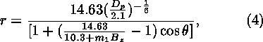
where m1 = 0 for northward IMF and m1
= 0.16 for southward IMF. The position Xprd
and Rprd (subscript pr denotes the
Petrinec and Russell [1996] model and superscript d denotes
dayside) are calculated by Xprd= r * cos(theta)
and Rprd = r * sin(theta).
The magnetopause location on the nightside was expressed in a different
functional form. For a given nightside position Xprn
(superscript n denotes nightside),
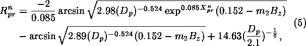
where m2 = 0.00137 for northward IMF and m2
= 0.00644 for southward IMF.
In their model, the dayside location does not depend on Bz
for northward IMF. On the nightside, the magnetopause location depends
weakly on positive Bz. For southward IMF, Petrinec
and Russell's [1996] flaring decreases rapidly as the dynamic pressure
increases. This model applies best when Dp > 1
nPa.
2.3. Comparisons Between the Two Models
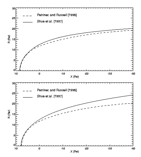
Figure 2 shows an example of the comparison
between Petrinec and Russell [1996] and Shue et al. [1997].
These two models give similar magnetopause location near the subsolar region.
They both predict a slightly smaller standoff distance for southward IMF
than for northward IMF. The predictions become different on the nightside.
For southward IMF, the Petrinec and Russell [1996] model has a less
flared tail magnetopause than the Shue et al. [1997] model.
The Shue et al. [1997] model predicts that the tail magnetopause
is more flared for southward IMF than for northward IMF.
| Figure 2. Comparison of Petrinec and
Russell [1996] and Shue et al. [1997]. (top) Northward
IMF (Bz = 5.0 nT and Dp = 8.0 nPa).
(bottom) Southward IMF (Bz = -5.0 nT and Dp
= 8.0 nPa). The vertical axis (R = sqrt(Y2+Z2))
is in aberrated GSM coordinates. |
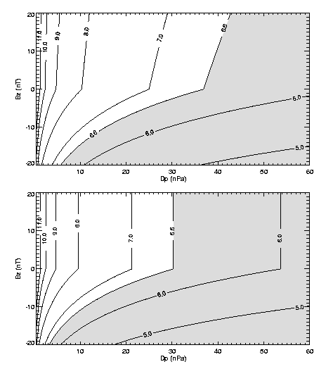
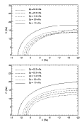
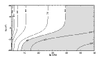
Figure 3 shows a general comparison of the
subsolar standoff distance r0 for these two models. The magnetopause
location relative to geosynchronous orbit is of particular interest for
space weather predictions because when the magnetopause moves within geosynchronous
orbit, satellites at that location are exposed to magnetosheath particles
and fields. The region within geosynchronous orbit is shaded in gray.
Figure 3 (top) shows the subsolar standoff
distance from Shue et al. [1997]; Figure
3 (bottom) is for Petrinec and Russell [1996]. We found
that r0 predicted by both models is within geosynchronous orbit
(less than 6.6 RE) for small Dp when the southward
IMF is extremely strong. Note that Figure 3
shows the equilibrium r0 for the corresponding values of Bz
and Dp. The magnetopause may oscillate around the
equilibrium value causing an uncertainty of about 0.5 RE near
the subsolar region [Song et al., 1988].
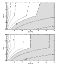
| Figure 3. Comparison of the subsolar standoff
distance r0 between (top) Shue et al. [1997] and (bottom)
Petrinec and Russell [1996]. The shaded (unshaded) region
shows that r0 is within (beyond) geosynchronous orbit. |
3. Application to the January Event
Using values of Bz and Dp observed
from the WIND satellite in Figure 1, we calculate
the magnetopause location as a function of time. A time delay of
24 min has been taken into account for the arrival of the solar wind at
the Earth. This time delay is calculated using the distance (~93
RE) between the WIND satellite and Earth (early on January 11,
1997) divided by the solar wind speed (~410 km/s) under the assumption
that the magnetopause is rigid and responds to solar wind conditions instantaneously.
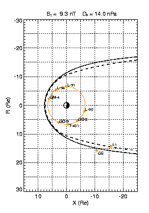
Figure 4 shows the locations of the magnetopause
and various satellites at 0100 UT (Bz = 9.3 nT and Dp
= 14.0 nPa). The solid and dashed curves represent the predictions
by Shue et al. [1997] and Petrinec and Russell [1996], respectively.
The difference between these two models is small on the dayside.
Since in situ observations from Geotail indicate that it was in the magnetosheath
during this time, both models succeed in the prediction.
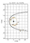
| Figure 4. Locations of the magnetopause
and satellites at 0100 UT on January 11, 1997. A solid curve is the
prediction by Shue et al. [1997]; a dashed curve is predicted by
Petrinec and Russell [1996]. Satellites are designated as follows:
L-90, LANL 1990-095; L-91, LANL 1991-080; L-94, LANL 1994-084; GO-8, GOES
8; GO-9, GOES 9; GM-4, GMS 4; T-401, Telstar 401; GE, Geotail; I-1, Interball
1. The vertical axis (R = sqrt(Y2+Z2))
is in aberrated GSM coordinates. |
We use these two models to calculate the distance between a satellite
and a model magnetopause along the normal to the boundary as a function
of time. Note that the solar wind aberration has been considered
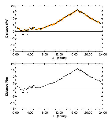
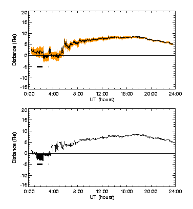
in these distance calculations. Figure 5
shows the calculated distances for the LANL 1994-084 satellite. A
positive (negative) distance indicates that LANL 1994-084 was in the magnetosphere
(magnetosheath).
| Figure 5. Distances between LANL 1994-084
and the magnetopause predicted by the two models as functions of time on
January 11: (top) Shue et al. [1997] and (bottom) Petrinec and
Russell [1996]. The distance is calculated as the smallest value
from the satellite to the predicted magnetopause. A negative distance with
a solid shading indicates that the satellite is in the magnetosheath.
A positive distance shows that the satellite is in the magnetosphere. The
uncertainty of the prediction estimated by Shue et al. [1997] is
shaded in gray. Thick horizontal bars below the curves indicate periods
when the satellite was in the magnetosheath according to the in situ measurements.
|
The predictions of these two models exhibit only
small differences for this satellite. LANL 1994-084 data show that the
satellite first crossed the magnetopause between 0152 and 0155 UT on January
11 and returned to the magnetosphere between 0217 and 0218 UT. There
was a very brief period within the magnetosheath between 0313 and 0316
UT [Thomsen et al., 1998]. Thick horizontal bars indicate
the periods when the satellite was in the magnetosheath. These two models
predict reasonably well the magnetopause location for this satellite, especially
when the uncertainty of the distance calculation (gray region in
Shue et al.) is taken into account. The uncertainty in the Shue et al.
model is estimated by using coefficients with their standard deviations
(by multiplying by a factor of 1/sqrt(3)) in Table 1 of Shue et al.
[1997] to calculate half of the difference between the maximum and minimum
magnetopause locations for each pair of Bz and Dp.
The reason for multiplying by 1/sqrt(3) is that Shue et al. [1997]
randomly sampled one third of the total points (rather than the total number)
to obtain the standard deviation. The uncertainty estimated when
one randomly samples K points from a data set including N
(> K) points is sqrt(N / K) times larger than the
real uncertainty when one randomly samples N points. We note
that the estimation error in the ``corrected'' quantity (by multiplying
by sqrt(N / K)) tends to increase with decreasing K.
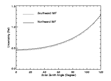
The uncertainty is calculated as functions of Bz, Dp,
and solar zenith angle. To demonstrate the uncertainty, we choose
Bz = -4 nT as an average value for southward IMF (dotted
curve) and Bz = 4 nT as an average value for northward
IMF (solid curve), as shown in Figure 6.
For Dp, an average value of 2 nPa is used. It can
be seen that the uncertainty increases rapidly with solar zenith angle,
and the uncertainty for the southward IMF is larger than that for the northward
IMF. This tendency is somewhat consistent with Figure
2 of Song et al. [1988], namely, the uncertainty could be mainly
associated with the magnetopause oscillations.
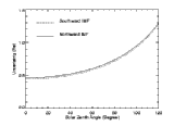
| Figure 6. Uncertainty of the Shue et
al. [1997] model versus solar zenith angle for southward and northward
IMF. |
The location of GMS 4 is more upstream than that of LANL 1994-084 during
the large dynamic pressure enhancement. The GMS 4 measurements indicate
that the satellite moved to the magnetosheath at 0115 UT (37 min earlier
than LANL 1994-084 did) and moved back to the magnetosphere at 0218 UT
(the same time as LANL 1994-084 did). Like LANL 1994-084, GMS 4 also
had a short excursion to the magnetosheath at 0315 UT. Figure
7 shows the distance from GMS 4 to the predicted magnetopause. Thick
horizontal bars in Figure 7 show the magnetosheath
periods. The two models predict reasonably well for this satellite.
| Figure 7. The distance from GMS 4 to the
predicted magnetopause in the same format as Figure
5. (top) Shue et al. [1997]. (bottom) Petrinec and
Russell [1996]. |
When Telstar 401 was lost at 1115 UT, the solar wind conditions had
returned to near normal values. The magnetopause had moved outward to 8
RE at the subsolar point, and Telstar 401 was far inside the
magnetosphere when the malfunction occurred.
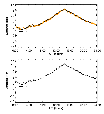
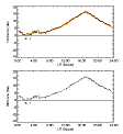
Figure 8 shows the distance to Geotail in
the same format as Figure 5. Visual inspection
of the particle distribution function data from the LEP instrument indicates
that Geotail was located in the magnetosheath at the beginning of the day,
made short excursions (lasting 1-4 min) into the magnetosphere at 0003,
0005, 0020, 0029, 0031, 0038, 0207, 0211, 0220, 0323, 0333, 0346, and 0428
UT, and finally entered the magnetosphere around 0547 UT. Although
Geotail was mainly located in the magnetosheath during the interval 0355
through 0547 UT, it was closer to the magnetopause than it had been before
0355 UT because Geotail observed very short intervals (lasting less than
~1 min) of magnetospheric ions (above ~1 keV). Thick horizontal bars
in Figure 8 show the magnetosheath intervals.
In Figure 8, the Shue et al. [1997]
prediction indicates that the distance changes sign from negative (solid
region) to positive (white region) around 0543 UT. This change is consistent
with the Geotail observations. Petrinec and Russell [1996]
predict Geotail crossed the magnetopause at 0345 UT and moved back and
forth between the magnetosphere and magnetosheath until 0541 UT.
Their prediction is partially consistent with the Geotail observations.
| Figure 8. The distance from Geotail to the
predicted magnetopause in the same format as Figure
5. (top) Shue et al. [1997]. (bottom) Petrinec and
Russell [1996]. |
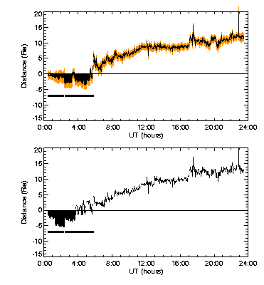
Figure 9 is a similar plot for Interball
1. Petrinec and Russell [1996] predict the magnetopause location
reasonably well. The magnetopause was within the error bar of the Shue
et al. [1997] prediction; however, significant differences of the magnetopause
crossing times indicate that Shue et al. [1997] needs improvement.
4. Improved Shue et al. Model
As shown in section 3, although the Shue et al. [1997] model
does an excellent job in predicting Geotail crossings, it has significant
room for improvement in order to predict Interball 1 crossings accurately.
Here we recall that the model was derived bivariantly based on observations
under average solar wind conditions. The complicated dependence on
the two variants may lead to some peculiar behavior when we extrapolate
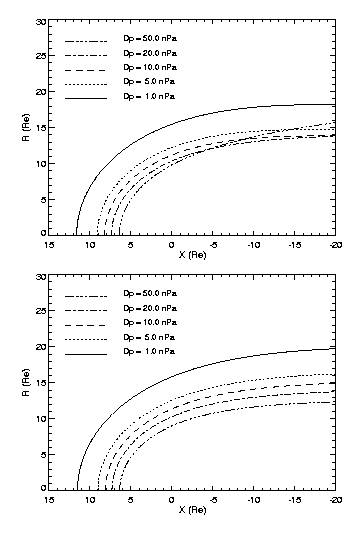
it to extreme conditions. Figure 10 (top)
shows the cross section of the magnetopause for Bz =
17 nT and various values of dynamic pressure for the Shue et al.
[1997] model.
| Figure 10. A demonstration of magnetopause
locations as functions of Dp with a fixed Bz
of 17 nT. (top) Shue et al. [1997]. (bottom) The improved
Shue et al. model. |
The magnetopause flares rapidly when Dp
is very high, which is peculiar as one would expect that the family curves
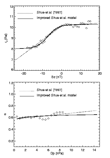
evolve smoothly. We investigate the reason why this happens by replotting
the observations (diamonds) and the linear fit of Shue et al. [1997]
(dotted curves) in Figure 11. We find
that the linear relationship extended to an extreme condition may exaggerate
the relationship. For example, the subsolar standoff distance may
approach zero when the IMF is extremely strong and southward, as shown
by the dotted curve in the top plot of Figure
11.
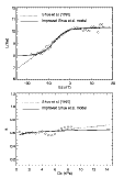
| Figure 11. (top) Value r0 as
a function of Bz. (bottom) Value alpha as
a function of Dp. The diamonds denote bin averages
of r0 and alpha derived from Shue et al. [1997]
using magnetopause crossings. Dotted and solid curves represent the
fitting results from Shue et al. [1997] and the improved Shue et
al. model, respectively. |
To improve our model, we fit r0 to a hyperbolic tangent function
for Bz and fit alpha to a natural
logarithmic function for Dp, which prevents r0
and alpha from reaching unphysical values for extreme cases, as
shown by the solid curves in Figure 11.
Note that Shue et al. [1997] expressed the relationship for northward
and southward IMF with two separate functions. The improved model
only uses a single function to represent the r0 dependence on
Bz. The natural logarithmic function for alpha
comes from substituting a power law of r0 versus Dp
into (1) and taking a natural logarithm of both sides of the equation to
obtain alpha = A + B ln(Dp), where
A and B are the factors to be determined. Using the new nonlinear
relationship, the best fit result gives


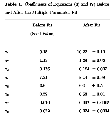
Combining (6) and (7) with the (5) and (7) of [Shue et al., 1997],
we obtain


where parameters a1 through a8 can
be optimized using the gradient search technique [Bevington, 1969].
The initial seed values of these parameters are shown in the first column
of Table 1. The final optimized values
and uncertainties are shown in the second column of Table 1.
The uncertainties are derived using the same Monte Carlo method used by Shue
et al. [1997]. We have run multiple-parameter fittings 200 times using
all dataset values which are sampled randomly each time, and points are
allowed to be sampled repeatedly. We obtain 200 sets of coefficients
and take their standard deviations as their uncertainties. The standard
deviation between the analytic and the observed values for the improved
model is 1.23 RE. The final expressions for our improved
model are


The improved Shue et al. model results are demonstrated in Figure
10 (bottom). The evolution of the magnetopause with Dp
becomes smooth. Using this improved formula, we recalculate the distance
from the predicted magnetopause to each satellite, as shown in Figure
12.
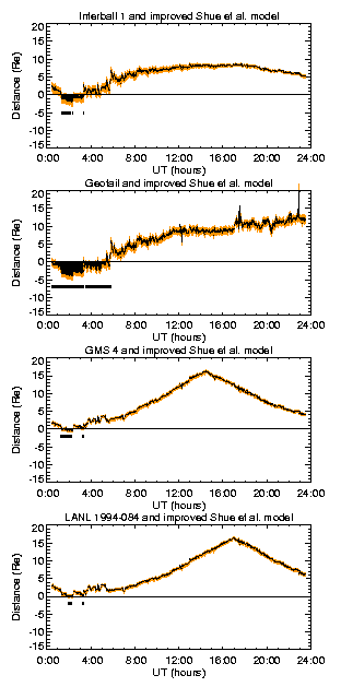
| Figure 12. Distances between the prediction
by the improved Shue et al. model to the Interball 1, Geotail, GMS 4, and
LANL 1994-084 satellites in the same format as Figure
5. |
The result leads to a significantly improved agreement with the
observations, especially with the Interball 1 observations. Finally,
we recalculate r0 versus Bz and Dp
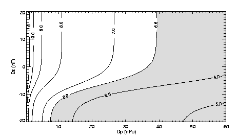
in Figure 13. Comparing with the top
plot of Figure 3, there is a significant
change in the region for extremely southward IMF and the contours become
smoother. Furthermore, the value of Dp needs to be at
least 7 nPa in order for a geosynchronous satellite to have a magnetopause
crossing, even when the IMF is extremely southward. This may be due
to the limited capability for reconnection to erode the magnetopause. Kuznetsov
and Suvorova [1997] reported some magnetopause crossings at synchronous
orbit. Their results are qualitatively consistent with our results, that
is, a smaller Dp is needed to have a geosynchronous crossing
when the IMF is southward than when the IMF is northward. However, quantitatively,
the two results are different. We note that they used hourly averages
of the solar wind measurements which tend to underestimate the peak values
of solar wind parameters.
| Figure 13. Standoff distance as functions
of IMF Bz and solar wind dynamic pressure Dp
derived from the improved Shue et al. model in the same format as Figure
3. |
5. Discussion and Conclusions
The differences between the two models are caused by the following factors.
First, the databases used in the two models are not the same. Second, the
basic functional forms of the magnetopause location are different.
The most important issue is how to handle the nightside magnetopause. The
function used by Petrinec and Russell [1996] gives an open magnetopause
on the nightside. Shue et al.'s [1997] functional form is mathematically
simple and can model both the open and closed magnetosphere. This
functional form provides the opportunity to describe how the magnetopause
evolves with different IMF orientations. Furthermore, the specific
dependence of the magnetopause on the upstream solar wind is different.
We have compared observations from several satellites with model predictions
by Shue et al. [1997] and Petrinec and Russell [1996] for
the January 11, 1997, event. During the January event, these two
models correctly predict the magnetopause crossings on the dayside.
It is therefore likely that either of these two models is able to provide
a reasonably accurate warning of dayside magnetopause crossings for geosynchronous
satellites. However, there are some differences in the predictions
along the flank. The Shue et al. [1997] model correctly predicts
the Geotail magnetopause crossings and partially predicts the Interball
1 crossings. The Petrinec and Russell [1996] model correctly predicts
the Interball 1 crossings and is partially consistent with the Geotail
observations.
The two models have treated the magnetopause as a rigid surface which
responds to the upstream changes instantaneously. However, the real
magnetopause is not rigid and will respond to the upstream changes dynamically,
especially under extreme conditions. The magnetopause will oscillate around
its equilibrium state. Therefore it is not expected that these models will
predict precisely every single magnetopause crossing under such conditions.
However, for the purposes of space weather forecasting, it is most important
to predict that magnetopause crossings will occur and not the precise number
of the crossings. As shown earlier, the level of the oscillations
is similar to the error bar in the model. Therefore, for the space
weather forecast, the magnetopause oscillation can be treated as a part
of the error bar.
We have improved the Shue et al. [1997] model by introducing
new functional forms to better represent the solar wind pressure effect
on the magnetopause flaring and the IMF Bz effect on
the subsolar standoff distance. The new functions provide a better implicit
description of the underlying physical conservation laws and lead to a
better agreement with the Interball 1 observations for this event.
Acknowledgements
This research was supported by Center of the Excellence (COE) program
of Ministry of Education, Science, Culture, and Sports of Japan.
The work at the University of Michigan was supported by NASA research grant
NAGW-3948 and NSF grant ATM-9713492. The work at UCLA was supported
by NASA under grant NAGW-3948 and by NSF under grant ATM 94-13081.
The work at National Central University was supported by the National Science
Council grant NSC 87-2111-M-008-008-AP8. G. Zastenker was partly
supported by Russian Foundation for Basic Research by grant 95-02-03998.
O. L. Vaisberg was supported in part under grant INTAS-93-2031. We
would like to thank B. J. Thompson, M. Peredo, N. Fox, and other persons
at NASA/GSFC who coordinated this event and collected related data for
the ISTP homepage. We are grateful to R. P. Lepping for magnetic
field measurements from WIND. Work at MIT was supported under NASA
grant NAG5-2839. The authors would like to thank S. M. Petrinec for
providing the program of his model. We want to thank E. C. Roelof and D.
G. Sibeck for their comments. We also want to thank T. Mukai and
Y. Saito of ISAS for using the LEP data from Geotail. We are indebted to
K. K. Khurana for the program of multiple-parameter fit. We thank
T. Obara of CRL for providing a list of crossings from GMS 4.
The Editor thanks T. Araki and another referee for their assistance
in evaluating this paper.
References
Aubry, M. B., C. T. Russell, and M. G. Kivelson, Inward motion of the
magnetopause before a substorm, J. Geophys. Res, 75, 7018, 1970.
Bevington, P. R., Data Reduction and Error Analysis for the Physical
Sciences, McGraw-Hill, New York, 1969.
Chapman, S., and V. C. A. Ferraro, A new theory of magnetic storm, I,
The initial phase, J. Geophys. Res., 36, 77, 1931.
Elsen, R. K., and R. M. Winglee, The average shape of the magnetopause:
A comparison of three-dimensional global MHD and empirical models, J.
Geophys. Res., 102, 4799, 1997.
Fairfield, D. H., Average and unusual locations of the Earth's magnetopause
and bow shock, J. Geophys. Res., 76, 6700, 1971.
Fairfield, D. H., Observations of the shape and location of the magnetopause:
A review, in Physics of the Magnetopause, Geophys. Monogr. Ser.,
vol. 90, edited by P. Song, B. U. \"O. Sonnerup, and M. F. Thomsen, p.
53, AGU, Washington D. C., 1995.
Ferraro, V. C. A., On the theory of the first phase of a geomagnetic
storm: A new illustrative calculation based on idealized (plane not cylindrical)
model field distribution, J. Geophys. Res., 57, 15, 1952.
Formisano, V., V. Domingo, and K.-P. Wenzel, The three-dimensional shape
of the magnetopause, Planet. Space Sci., 27, 1137, 1979.
Gosling, J. T., M. F. Thomsen, S. J. Bame, R. C. Elphic, and C. T. Russell,
Observations of reconnection of interplanetary and lobe magnetic field
lines at the high-latitude magnetopause, J. Geophys. Res., 96, 14,097,
1991.
Howe, H. C., and J. H. Binsack, Explorer 33 and 35 plasma observations
of magnetosheath flow, J. Geophys. Res., 77, 3334, 1972.
Kartalev, M. D., V. I. Nikolova, V. F. Kamenetsky, and I. P. Mastikov,
On the self-consistent determination of dayside magnetopause shape and
position, Planet. Space Sci., 44, 1195, 1996.
Kuznetsov, S. N., and A. V. Suvorova, Magnetopause shape near geostationary
orbit (in Russian), Geomagn. Aerono., 37(3), 1, 1997.
Petrinec, S. M., and C. T. Russell, An empirical model of the size and
shape of the near-Earth magnetotail, Geophys. Res. Lett., 20, 2695,
1993.
Petrinec, S. M., and C. T. Russell, Near-Earth magnetotail shape and
size as determined from the magnetopause flaring angle, J. Geophys.
Res., 101, 137, 1996.
Petrinec, S. M., P. Song, and C. T. Russell, Solar cycle variations
in the size and shape of the magnetopause, J. Geophys. Res., 96,
7893, 1991.
Roelof, E. C., and D. G. Sibeck, Magnetopause shape as a bivariate function
of interplanetary magnetic field Bz and solar wind dynamic
pressure, J. Geophys. Res., 98, 21,421, 1993.
Shue, J.-H, J. K. Chao, H. C. Fu, C. T. Russell, P. Song, K. K. Khurana,
and H. J. Singer, A new functional form to study the solar wind control
of the magnetopause size and shape, J. Geophys. Res., 102, 9497,
1997.
Sibeck, D. G., R. E. Lopez, and E. C. Roelof, Solar wind control of
the magnetopause shape, location, and motion, J. Geophys. Res., 96,
5489, 1991.
Song, P., and C. T. Russell, Model of the formation of the low-latitude
boundary layer for strongly northward interplanetary magnetic field, J.
Geophys. Res., 97, 1411, 1992.
Song, P., R. C. Elphic, and C. T. Russell, ISEE 1 and 2 observations
of the oscillating magnetopause, Geophys. Res. Lett., 15, 744, 1988.
Sotirelis, T., The shape and field of the magnetopause as determined
from pressure balance, J. Geophys. Res., 101, 15,255, 1996.
Thomsen, M. F., J. E. Borovsky, D. J. McComas, R. C. Elphic, and S.
Maurice, The magnetospheric response to the CME passage of Jan. 10-11,
1997, as seen at geosynchronous orbit, Geophys. Res. Lett., in press,
1998.
 Back to CT Russell's page
 More On-line Resources
Back to the SSC Home Page