Ogo 5 Observations of Upstream Waves in the Interplanetary Medium: Discrete Wave Packets

C. T. Russell, D. D. Childers,* and P. J. Coleman, Jr.*

Abstract. One class of waves observed in the interplanetary medium within several earth radii of the earth's bow shock consists of discrete wave packets with amplitudes that are a significant fraction of the background magnetic field. In the spacecraft frame, these wave packets have periods of about 2.5 sec. grow rapidly in time and decay more slowly, and are left-handed with respect to the magnetic field. By using the measured solar wind density and cold plasma dispersion theory, however, we show that these wave packets must be right-handed in the plasma frame at frequencies from about 2 to 4 times the proton gyrofrequency. The propagation vector of these waves is found to point away from the earth's bow shock and to lie between the solar wind flow direction and the average spiral field. The waves are being carried away from the sun by the solar wind, since their velocity is less than the solar wind speed, but they appear to be associated with the intersection of the field line with the earth's bow shock. Since they must be generated in the solar wind plasma, this generation may be caused by the presence of particles streaming upstream from the shock.

INTRODUCTION

The magnetic field observed upstream from the earth's bow shock in the interplanetary medium is often irregular or turbulent in appearance [Fairfield, 1969]. The observed fluctuations may be produced either by a source that generates a broad spectrum of frequencies with random phases or by a superposition of waves from independent sources. In the second case, each wave packet could be well defined, but the mixture of many such packets would result in a random wave field.

Even if we could measure the field fluctuations in the rest frame of the plasma, it would be difficult to interpret them because of the dispersive nature of a plasma, i.e., because the propagation velocity depends on frequency and angle of propagation to the magnetic field, and these can vary from wave to wave. In practice we are faced with an additional difficulty resulting from the fact that the measurements are necessarily made on a probe that is essentially at rest relative to the earth rather than to the plasma. The plasma streams past the probe at the solar wind velocity, which is from the same order to an order of magnitude greater than the wave velocity.

Fortunately, there are occasions when the wave fields are dominated by regular periodic oscillations. Examples of such waves have previously been reported by Heppner et al. [1967] (their Figure 24), Simmons and Coleman [1968], and Fairfield [1969] (his Figure 2). For such waves it is somewhat easier to make meaningful comparison with theory. In this paper we examine one type of discrete wave phenomenon by using the magnetic field data from the UCLA fluxgate magnetometer on Ogo 5.

EXPERIMENT

To study these waves, we analyze data obtained by the UCLA fluxgate magnetometer carried on board the Ogo 5 satellite, which has an apogee of 24 earth radii. The experiment is described in detail by Aubry et al., [1971]. Briefly, the magnetometer measures the three orthogonal vector components of the magnetic field with a digital window of 0.125 nT, at rates of up to 56 samples of the vector field per second. For various reasons the absolute accuracy is somewhat less than the precision, averaging about 1 nT uncertainty in each of the vector components. The accuracy is checked by intra-comparison with the GSFC magnetometer on the same spacecraft.

Use will also be made of the solar wind parameters obtained by the JPL solar wind experiment provided by M. Neugebauer. A description of this experiment has been given by Neugebauer [1970].

REGULAR WAVETRAINS

Although the waves upstream from the bow shock are often irregular, there are times when they are quite regular. Figure 1 shows 3 min of data taken at such a time. The waves have periods of about 30 sec and peak-to-peak amplitudes of about 5 nT. In his Figure 2, Fairfield [1969] shows a very similar train of waves. The digitization window is a factor of 2 smaller in this experiment, and the data in Figure 1 were sampled 18 times faster than the data from Imp 4. However, such improvements do not in themselves add to our knowledge of the character of these low-frequency waves.

Figure 2 shows a regular wavetrain with a period of 3.2 sec. Again, the amplitude is roughly 5 nT. Such waves could not be resolved with the sampling rate of the Imp 4 magnetometer. The UCLA Ogo 5 magnetorneter, however, was not the first to detect such wave packets in the interplanetary medium. Figure 24 of Heppner et al. [1967] shows such a wave packet. Unfortunately, the Ogo 1 spacecraft was spinning with unknown orientation and the magnetometer did not deploy properly, so only one component could be studied.

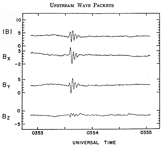
The occurrence of wave packets at these frequencies in an otherwise quiet magnetic field as in this example is extremely rare. Figure 3 shows the usual situation. Here the discrete wave packets with periods of about 1.5 sec occur in conjunction with an irregular train of waves at much longer periods, roughly 20 sec. The amplitudes of both sets of waves are similar and, in fact, are comparable to the field magnitude. In addition to the three well-defined wave packets, what may be termed incipient wave packets are seen at 0857: 15, 0859: 15, and 0900. In what may be a variant of the phenomenon shown in Figure 3, the low-frequency fluctuations can be accompanied by continuous higher frequency waves. This situation is shown in Figure 4. It is difficult to separate individual wave packets in such cases. Furthermore, examples of such behavior of the field are rare in the sample studied, and the waves in these cases have smaller amplitudes than the discrete wave packets illustrated in Figures 2 and 3. Since the waves in Figures 2 and 3 are so well defined and regular in appearance, we can measure their direction of propagation with only an ambiguity in sign and their frequency and sense of polarization in the satellite rest frame. Knowing these quantities plus the solar wind flow velocity and number density, we can in principle determine the wave frequency in the plasma rest frame and can determine the possible wave-plasma interactions.

 

Fig. 1.The magnitude of the field and three vector components in the spacecraft coordinate system illustrating an occurrence of quasi-sinusoidal waves at low frequencies in the interplanetary medium on March 10, 1968. The field magnitude is measured in nanoTeslas and the time is in hours and minutes. The satellite was at a radial distance of 20.43 RE and a sun-earth-satellite angle of 65.3o.

 

Fig. 2.An occurrence of an isolated discrete wave packet on March 14, 1968, while the satellite was at 21.9 RE and at a sun-earth-satellite angle of 49.5o.

Therefore, they appear to be prime candidates to lead us to a better understanding of the wave-plasma interactions in this region upstream from the bow shock, and we concentrate our analysis in this paper on such events. Analysis of the statistical properties of these regions, such as power spectral analysis, will be deferred to a later paper.

 

Fig. 3.Discrete wave packets occurring in association with irregular low-frequency waves on March 10, 1968, while the satellite was at 19.1 RE and at a sun-earth-satellite angle of 67.5o.

 

Fig. 4.Continual high-frequency waves simultaneous with quasi-sinusoidal low-frequency waves on March 8, 1968, while the satellite was at 21.9 RE and at a sun-earth-satellite angle of 61.3o.

AVERAGE PROPERTIES OF THE DISCRETE WAVE PACKETS

Before examining some of these waves in detail, we first look at their average properties, in particular their amplitude, period, and duration. To determine these average properties, 42.5 hours of high-resolution waveform data were scanned, representing a wide range of solar wind magnetic activity. Since only the initial orbits of Ogo 5 were available for this study, all events were obtained on the dawn side of the earth-sun line. Only the 7- or 56-sample per sec data were used. On the original plots every available point was plotted, with 100 points per inch on the horizontal scale and 10 nT per inch on the vertical scale. An occurrence of a discrete wave packet was counted if the maximum peak-to-peak amplitude of a wave was greater than 1 nT, if it lasted 2 or more cycles, and if it had a well-defined period of between 0.72 and 7.2 sec. During these 42.5 hours only 64 events satisfied these criteria, or about one every 40 min on the average. However, they are not randomly spaced throughout the data but tend to occur in groups, and as seen in Figure 3, they tend to occur in the presence of the longer period waves, which have been shown to be associated with the intersection of the magnetic field line with the earth's bow shock [Fairfield, 1969].

Nevertheless, the presence of long-period fluctuations was not a sufficient condition for the presence of the discrete wave packets, because the longer period fluctuations often occur without such wave packets, but it is almost a necessary condition. Of the 64 events only 5 occurred when there were no significant field oscillations at low frequencies (<O.l Hz). One of these 5 events is shown in Figure 2. Since these waves generally occur in conjunction with the low-frequency waves that occur when the field intersects the shock, in general these waves must also be related to intersection of the field line with earth's bow shock.

The amplitude, duration, and period of each of these events were also noted. The amplitude of the largest component of the wave in the spacecraft coordinate system was measured at the maximum of the event. Figure 5 shows the distribution of occurrence of peak-to-peak amplitudes. Only 2 events had maximum amplitudes of greater than 10 nT. The average peak-to-peak amplitude was 4.5 nT. This maximum amplitude also generally occurred at the start of the wave packet. Only 4 events appeared to have longer growth times than decay times. (In this section the terms 'growth' and 'decay' refer to the increase and decrease in amplitude, respectively, measured in the reference system of the magnetometer). An example of this behavior is shown in Figure 6. Only 3 events had a constant amplitude throughout their duration. Of the 64 events, 57 grew rapidly to maximum amplitude and then decayed more slowly. The waves in Figures 2 and 3 display this typical behavior.

 

Fig. 5.The per cent occurrence per 1-nT interval of the maximum peak-to-peak amplitude of the largest magnetic field component for 64 discrete wave packets. Only wave packets of maximum amplitude greater than 1 nT, duration greater than one cycle, and with periods from 0.72 to 72 sec were considered.

Figure 7 shows the percent occurrence of periods for these events. A characteristic period was defined for each event, but often the frequency changed throughout the event. This characteristic frequency is an average over the first 2 cycles. We see that typically these waves have periods of about 2.5 sec, although some wave packets bad periods up to 7 sec, which was the longest period considered in this study. The absence of events at short periods at ~1 sec is not a selection bias. Figure 8 shows the distribution of duration for these events. Very few packets were long-lived. Over 60% of the events lasted only 2 or 3 cycles.

We can also use the plots of the waveforms to measure the polarization. This could be done unambiguously for 57 events. Each of the wave packets that occurred in conjunction with low-frequency waves and that reached a maximum amplitude during the first half of the duration of the event was left-handed polarized with respect to the field as measured in the spacecraft frame of reference. On the other hand, the 2 waves that grew slowly and decayed rapidly and whose polarization could be measured from the plots were both right-handed. Also, all 5 events that occurred in the absence of any low-frequency waves were right-handed.

Fig. 6.A discrete wave packet with anomalous time behavior occurring on March 10, 1968, while the satellite was at 22.0 RE and at a sun-earth-satellite angle of 62.6o.

In general, then, these packets are left-handed with respect to the field as measured in the spacecraft frame of reference. They represent a large perturbation in the interplanetary field (average maximum peak-to-peak amplitude, 4.5 nT) but are infrequent. They have an average frequency of 0.4 Hz and last only a few cycles.

PRINCIPAL AXIS SYSTEM

For a plane wave in an infinite homogeneous medium, the field of the wave as measured by an observer oscillates in a plane. In general the field perturbation is not circular in this plane but is elliptical, and thus usually we can find a direction of maximum perturbation and minimum perturbation in this plane. One of the two directions normal to this plane is parallel to the propagation vector, that is, the direction of the phase velocity of the wave. In the ideal case, there are no fluctuations in this direction.

Fig. 7.The per cent occurrence per 0.72-sec interval of the periods of the discrete wave packets.

Fig. 8.The per cent occurrence per cycle of the duration of the discrete wave packets.

The technique used to find these three orthogonal directions for a wave is identical to that used by Sonnerup and Cahill [1967] to find the direction of the normal to the magnetopause. In this case, however, we high-pass filter the data to remove any possible effect of long-period waves on the analysis. Even though the waves we are examining dominate the fluctuations at these times, since we are analyzing a band of frequencies, and because we are not necessarily dealing with plane waves, there is still some power in the direction normal to the plane of the oscillation. For all cases of discrete waves studied, this power is small compared with the power along the other two axes, generally about 1%.

In practice, this analysis is simply an eigenvalue problem on the variance matrix of the measured field values. The resulting eigenvalues are proportional to the power along each of three principal axes (the eigenvectors). The eigenvector associated with the minimum eigen-value is either parallel or antiparallel to the direction of propagation. We cannot determine the sign of the propagation vector from this analysis alone; we require at least one component of the electric field of the wave to unambiguously determine this sign. In the following analysis, we define the direction associated with the largest eigenvalue to be the X axis, the direction associated with the intermediate eigenvalue to be the Y axis, and the direction associated with the smallest eigenvalue to be the Z direction.

Figure 9 shows a hodogram of one of these discrete wave packets in the plane of the oscillation obtained by using this technique. The amplitude of the wave increases rapidly to a maximum and then decays over the next 6 cycles. The wave is elliptically polarized but is not far from being circularly polarized. The ratio of the eigenvalues indicates that the power along the direction (Z) normal to this plane is about 2% of that along the X or Y axis. The average unfiltered vector field over the duration of this wave in this coordinate system is (6.0, 1.4, -3.1) nT. Thus, the wave is propagating at a large angle, 62^o, to the field. We also see from this figure that the wave is left-handed with respect to the field in the rest frame of the satellite.

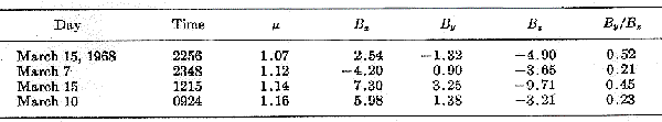
Figure 10 shows the hodogram in the principal axis system for another discrete wave packet. The wave has been split into two parts at the point marked 'A' for clarity. This wave completes 2 cycles before reaching maximum amplitude and then decays over 5 cycles. It is also more circular than the previous example. Here the power on the Z axis is 1% of the power on the X or Y axes. The average field in the principal axis system of the wave is (2.54, -1.32, -4.90) nT. Thus, this wave is propagating at 30^o to the magnetic field. Again the wave is left-handed, relative to the mean field, as measured by the magnetometer.

Figure 11 shows a third wave. In this example the wave remained at an almost constant amplitude for 6 oscillations and for clarity has been split into four parts. Again the time required to reach maximum amplitude is less than the time for decay. Here the average unfiltered field is (-1.4, 1.7, 6.2) nT, indicating a propagation angle of 20^o. This wave is even more circular than in the previous example.

In fact the directions of the X and Y axes here are essentially arbitrary, since the difference in the eigenvalues associated with the X and Y axes is small. As before, this wave is apparently left-handed. We note that this wave packet occurred only 3 min after the wave in Figure 10.

 

Fig. 9.A hodogram of the oscillating field due to a discrete wave packet in the principal axis system. The low-frequency fluctuations and background magnetic field have been removed with a high-pass filter. The average magnetic field in this system averaged over the duration of the wave packet and the ratio of the eigenvalues obtained in the analysis of the variance matrix are given in the figure. The satellite was at a radial distance of 19.3 RE and at a sun-earth-satellite angle of 67.1o.

Another feature of the waves is an apparent increase in frequency throughout the duration of the wave packet. This can be seen by close inspection of Figures 9, 10, and 11 but is shown more clearly in Figure 12, where the period as a function of time is plotted for the 3 illustrated events plus 1 additional event. In all cases there is a decrease in the wave period with time. This decrease is most rapid at the beginning of the event.

There is also consistency in the direction of propagation obtained from the principal axis technique. Although the propagation vector can be at a wide variety of angles to the magnetic field, it tends to lie between the earth-sun line and the typical spiral angle of the interplanetary magnetic field. This is illustrated in Figure 13, where we have plotted the projection onto the ecliptic plane of the unit vector parallel to the propagation vector for 7 normal examples of the discrete wave packets plus the 2 anomalous examples illustrated in Figures 2 and 6. To minimize possible errors in the determination of the direction of propagation, these 9 events had both larger amplitudes and longer durations than the means of the distribution in Figures 5 and 8. The directions of propagation have been chosen to point toward the sun (positive X component), but in fact we have an ambiguity in sign. Furthermore, all cases were obtained on the dawn side far above the ecliptic plane.

 

Fig. 10.The hodogram of a discrete wave packet in the principal axis system. The satellite was at 23.0 RE and at a sun-earth-satellite angle of 63.5o. The wave packet is shown in two parts, broken at point A for clarity.

 

Fig. 11.The hodogram of a discrete wave packet in the principal axis system. This event occurred only 3 min after the event of the previous figure. This wave has been divided into four parts for clarity.

Figure 13 shows that the direction of the phase velocity of 8 of the 9 wave packets was between the earth-sun line (the X axis) and the typical 45^o spiral angle. By projecting the direction of propagation into the plane defined by the flow direction of the solar wind and the direction of the magnetic field, it was verified that in individual cases the propagation vector usually does he between these two directions. Of the 9 instances, only 2 did not lie between the solar wind flow direction and the magnetic field, and in these the propagation vector was within 6^o of lying between them. This difference is within experimental error.

Also, we see from Figure 13 that these directions were within 45^o of the ecliptic plane, and 8 of the 9 vectors were directed upward. The one exception is indicated by an open circle. This tendency for propagation vectors to be directed upward, out of the ecliptic plane, may be associated with the fact that the satellite ranged from 12 to 16 R_E above the ecliptic plane for these events. Unfortunately this cannot be tested by selecting events at different locations because Ogo 5 did not sample the region near the ecliptic plane in the interplanetary medium during its first year of operation.

The eigenvalue or principal axis technique allows us to determine the propagation vector of the waves. The waves are found to be propagating at a wide variety of angles to the field, but typically the phase velocities lie within 45^o of the ecliptic and between the earth-sun line and the usual spiral angle; however, they are usually circularly or only slightly elliptically polarized. Most often the waves appear left-handed with respect to the field as measured in the spacecraft rest frame and appear to increase in frequency during the event. The waves are undoubtedly severely Doppler-shifted, however, because of the flow of the solar wind plasma, in which the waves propagate, relative to the spacecraft. In addition to changing the apparent frequency of the waves, this Doppler shifting can actually reverse the apparent polarization of the waves. In this regard, it should be noted that the directions of propagation of the 2 right-handed waves plotted in Figure 13 are among the furthest from the solar wind flow direction, and therefore these waves may be less affected by Doppler shifting than the other events. Next we investigate the effects of this Doppler Shifting and estimate the wave frequency in the plasma rest frame.

ACTUAL WAVE FREQUENCY AND POLARIZATION IN THE PLASMA FRAME

The Doppler shift of a wave in the solar wind is determined by the component of the solar wind velocity along the propagation vector of the wave. If this component is negative, i.e., if the wave propagates against the solar wind, and if this component is greater in magnitude than the wave phase velocity, then the wave will be carried past the satellite, which is essentially at rest relative to the earth, and the polarization of the wave will be reversed. Thus, a right-handed wave can appear left-handed if it is moving upstream away from the bow shock. Waves propagating in the same direction as or against the solar wind, but at very large angles to it, will not change polarization although their apparent frequencies will be altered.

With this experiment, we can obtain the direction of propagation with an ambiguity in sign and the apparent sense of rotation. We have the direction and magnitude of the background field. With the addition of information from the JPL solar wind experiment, we have the solar wind velocity, direction, number density, and proton temperature. In principle, it is then possible to find from theory the phase velocity as a function of frequency for the specific solar wind conditions, to add the amount of Doppler shifting that the solar wind would cause at each frequency, and then to see which frequencies would be Doppler shifted to the observed frequency and polarization. This would result in a small number of possible true frequencies. If the waves are source free, we could then compare the predicted ellipticity of the waves with the observed ellipticity to give an unambiguous identification of the wave.

 

Fig. 12.The variation in the period of the waves over the duration of four wave packets measured in terms of both data samples per cycle and seconds.

 

Fig. 13.The projection onto the ecliptic plane of the unit vector in the direction of propagation of nine wave packets. The X and Y axes are the usual solar ecliptic directions: X toward the sun and Y to dusk. The angle out of the ecliptic plane is indicated by the distance of a point from the unit circle. Circles indicating angles of 0o, 30o, 50o, and 70o to the ecliptic plane have been drawn. Wave packets with normal behavior are represented by circles. A closed circle indicates a propagation vector pointing above the ecliptic plane, and an open circle indicates a vector pointing into the ecliptic plane. The crosses represent the two anomalous cases shown in Figures 2 and 6. Both these wave packets had propagation vectors pointing above the ecliptic plane. The sign of the propagation vector was chosen by assuming that all wave packets were propagating upstream.

The dispersion relation for large-amplitude waves in a hot multicomponent plasma such as the solar wind is very complicated. Hence we shall treat the solar wind as a cold multicomponent plasma, and we further assume that the wave fields are much smaller than the background field, which we have seen from Figures 2, 3, and 6 is not true. This will enable us to obtain at least approximate solutions.

For small-amplitude freely propagating plane waves in a homogeneous cold plasma the ratio of the amplitudes, in the two orthogonal directions in the plane of the wave, can be shown to be [Russell, 1968]

 

Fig. 14.The variation of ellipticity as a function of angle of propagation to the magnetic field from cold plasma theory for various multiples of the proton gyrofrequency, W p, in a plasma of 5 electrons, 45 protons and 0.25 alphas per cm3 and with a magnetic field of 5 nT. The values obtained from measurements are also shown.

Before examining the analysis of specific cases, we can compare the functional relations predicted by equation 1 with those in the data. Figure 14 shows the angle of propagation of 7 events plotted versus the ratio of the major to minor axis of the perturbation ellipse of the wave. The lines represent the size of this ratio for different frequencies in a cold plasma, chosen to represent. typical solar wind conditions, composed of 4.5 protons, 0.25 alphas, and 5 electrons per cm³ in a field of 5 nT. The measured ellipticity is the square root of the ratio of the two largest eigenvalues. The ends of the error bars are the values obtained by adding and subtracting the minimum eigenvalue from the maximum.

The ends of the error bars on the angle of propagation represent the angles of propagation obtained by increasing and decreasing the amplitude of the largest component of the average field in the principal axis system by 1 nT.

To the accuracy of the plot, both right- and left-handed waves at the same frequency have the same ellipticity as a function of angle of propagation. Thus, the curves for W _p/8, W _p/4, W /2, and W _p, are equally valid for left- and right-handed waves. The curve labeled W _p/2 and W _p, is actually for a frequency slightly below these frequencies, since these frequencies are limits of propagation in a cold plasma containing alphas and protons.

We see that at high frequencies waves are nearly circular for all but larger angles of propagation, but at low frequencies the waves become very elliptical at smaller angles. The observed waves fall in the middle of the range, and in fact agree well with the expected behavior of waves from W _p to 4W _p. In a cold plasma, only right-handed waves can propagate at these frequencies. Thus, to the extent that the cold plasma equations are valid, Figure 14 indicates that the discrete wave packets are right-handed waves at about 2 to 4 times the proton gyrofrequency.

We have a further test of the sense of polarization of the waves from equation 1. It was stated above that in general left-handed waves have a maximum perturbation field normal to the plane containing the background field and the direction of the propagation and right-handed waves had a maximum in that plane. Thus, in an ideal case the background field measured in the principal axis system would have zero X component for a left-handed wave and zero Y component for a right-handed wave.

Of course, we cannot apply this test for circularly polarized waves. Table 1 shows the ratio of B_y, to B_z for the 4 cases in Figure 14 with an ellipticity greater than 1.05. In all 4 cases, this ratio is less than unity and in fact is equal to or less than 0.5. Again the results are consistent with the result we would expect for right-handed waves in a cold plasma. In fact, the size of B_y, in all these cases is to be expected from the two sources of possible error, namely inaccuracy in the determination of the orientation of the X and Y axes about the direction of propagation due to 'noise' and the inaccuracy of the determination of the absolute value of the field.

It is important to emphasize that, although these two tests both depend on equation 1, they are independent tests because our first test involved the angle of propagation determined by (B_x² + B_y²)^½ and B_z whereas our second test involved the ratio of B_y to B_z.

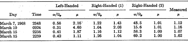
Finally, we attempt the analysis indicated at the beginning of this section, using the measured solar wind parameters and the derived wave properties to find the possible true frequencies in individual cases. At first this appears to be a more profitable exercise than the two just performed. However, the results of such an analysis are subject to both many experimental errors and theoretical assumptions. First, we have errors in the magnitude of the field and its direction relative to the direction of the propagation vector. Second, there are errors in the solar wind density, composition, flow velocity, and flow direction. Third, we must assume a cold plasma and small-amplitude waves. The actual phase velocity may be greater or less than this value, depending on the size of the proton and electron pressures and pitch angle anisotropies [Kennel and Scarf, 1968]. Finally, we assume a steady state while the wave is in progress. Usually, however, the field and the plasma conditions are changing during these events. Considering this, we used the average measured field, a characteristic frequency for each event, the measured propagation direction, the measured solar wind density, and flow velocity and have computed the possible true frequencies for four events. These are presented in Table 2.

Table 1. The Average Magnetic Field in the Principal Axis System for the Four Wave Packets with m >1.05

In general, if we measure a left-handed wave in the satellite system at the observed apparent frequencies there are three possible waves. One, is a left-handed wave below the proton gyro-frequency propagating with the solar wind; one is a right-handed wave just above the proton gyrofrequency propagating against the solar wind; and one is a right-handed wave far above the proton gyrofrequency. The third solution occurs just below the frequency at which the component of the solar wind flow velocity parallel to the phase velocity equals the phase velocity.

By examining Table 2 we see that the left-handed solution is on the average about 0.4 W _p, the first right-handed solution is about 1.2 W _p, and the second right-handed solution is above 50 W _p. Since these results are subject to many sources of error, the first right-handed solution is in agreement with our previous two tests. The ellipticities both predicted and observed are also listed in Table 2, and it is seen that the ellipticity predicted for the two right-handed waves agrees much better with the observations than does the ellipticity of the left-handed waves. Furthermore, the apparent agreement of the high-frequency solution is solely due to the fact that all the predicted ellipticities are close to unity.

In summary, our three tests for the sense of polarization agree that the waves are right-handed with respect to the field in the plasma rest frame. Since we must use cold plasma theory, the determination of the frequency in this frame is somewhat imprecise, but it appears that the frequency lies between about 2 and 4 W _p. For the waves to appear left-handed in the satellite frame but be right-handed in the plasma frame, the waves must be propagating toward the sun in the plasma frame but be carried away from the sun by the solar wind.

DISCUSSION

Our purpose here was to study a wave phenomenon occurring in the region upstream from the earth's bow shock to provide a better understanding of the physics of this region. The discrete wave packets, examined for this purpose, would appear to allow the most unambiguous determination of wave properties because of their repeatability and distinct features. Even so, part of our analysis has had to depend on the assumption that certain properties predicted by cold plasma theory for small-amplitude plane waves will also be possessed by these large-amplitude wave packets propagating in a disturbed hot plasma. Nevertheless, we will assume henceforth that our analysis is correct, that these waves are right-handed waves propagating against the solar wind, and that their frequency in the solar wind frame is of the order of 2 times the proton gyrofrequency.

Table 2. The Three Possible Frequencies in the Plasma Frame. That Would Give an Apparent Left-handed Wave at the Observed Frequency in the Satellite Frame*

*Obtained by using the cold plasma dispersion relation and the measured solar wind parameters. The frequencies are given in terms of the measured proton gyrofrequency W _p, The theoretical value of m is given for each of the three frequencies together with the observed value of m .

The physically important questions about these waves are: where were they produced, what mechanism generated the waves, and what effects do the waves have on the plasma once they have been generated? We can partly answer the question about the location of generation rather quickly. We have not examined the spatial occurrence of these waves thus far, but the fact that these waves are found several earth radii from the shock entirely eliminates the possibility that these particular waves were generated at the shock and propagated to the satellite. This is true because at the frequencies of these waves, again using cold plasma theory, the group velocity is about 1/3 of the solar wind velocity. At such a group velocity the maximum angle to the solar wind in the shock frame at which the wave packet will appear to propagate is 19.5^o. On the other hand, the angle the shock makes with the solar wind varies from 90^o at the subsolar point to about 30^o at the dawn-dusk line.

Thus, the waves would be blown into the magnetosheath as soon as they were created anywhere above the dayside hemisphere if they were generated at the shock. To explain our observations in terms of generation at the shock would require group velocities equal to 95% of the solar wind velocity in the most extreme case measured so far. We do not expect that the temperature corrections to the group velocity would be this large. Thus the waves must be generated in the interplanetary medium itself.

The source of energy for these waves may be the energy of the solar wind bulk flow, the thermal motion of its constituents, or its magnetic field. Since it appears that these waves are present only when the shock is sensed by the interplanetary flow, these waves do not appear to be associated with an instability deriving energy from one of these quantities, as they are distributed far from the shock front.

The solar wind must have some information about the presence of the shock because we find it disturbed in these regions. Thus it is apparent that the usual solar wind distribution functions are either altered by this source of information, thereby paving the way for an instability, or that this source of information is itself unstable. An example of the first would be a wave that could propagate upstream against the solar wind; an example of the second would be particles 'reflected' by the shock [Anderson, 1968, 1969; Asbridge et al., 1968; Frank and Shope, 1968].

We first consider the possibility that a wave generated at the shock could propagate upstream, thereby changing the quiescent solar plasma, which then by some mechanism radiates the waves seen here. Initially this appears reasonable because we almost always see these wave packets in association with other low-frequency waves. However, these low-frequency waves appear left-handed in the satellite frame [Fairfield, 1969]. To have a group velocity greater than the solar wind streaming velocity the waves must be right-handed, but to appear left-handed the phase velocity must be less than that of the solar wind streaming velocity. This is possible for whistler mode waves because the group velocity can be up to twice the phase velocity. However, Fairfield [1969] reports that the velocity of this information is 2.7 ± 0.4 times the solar wind velocity. If this velocity did represent the group velocity of a whistler wave, then its phase velocity would also be greater than the solar wind velocity and there would be no polarization reversal. Hence the low-frequency waves cannot be generated at the shock, and the source of information must be in 'reflected' particles.

In retrospect, it is quite reasonable that reverse flow particles exist, and in fact Axford [1966] mentioned this possibility. If the shock front traps a fraction of the solar wind particles and the particles move in the direction of the interplanetary electric field, the particles will be accelerated. (See, for example, Sonnerup [1969].)

Little is known about the typical energy spectrum or the pitch angle distribution of the 'reflected' particles. Furthermore, it is difficult to hypothesize reasonable values for them until we better understand the reflection process and the nature of the shock. However, if the shock energizes electrons and protons in the same proportion relative to their streaming velocity or even gives them the same absolute increment of energy in the reflection process, we expect protons to be more unstable than electrons. For the electrons, the high thermal energy, relative to the streaming energy, will tend to smooth out any peaks in the distribution functions, but for the protons there will exist two well-defined peaks in velocity space, one for the incident solar wind protons and one for the reflected protons.

It is also difficult to predict the spatial distribution of these reflected protons, whether they form beams with sharp edges or occur in a broad homogeneous region. If they occur in sharply bounded regions, say flux tubes or filaments, the boundaries may be unstable to gradient-associated instabilities or drift waves. Whatever the source of these waves is, it must be capable of producing coherent wave packets at well-defined frequencies. For this reason, the theory developed by Barnes [1970] to explain the low-frequency turbulence cannot strictly apply to these waves.

Given the existence of these waves and their properties, we can determine the possible wave-particle resonances. These resonances could either lead to net growth or to damping of the waves, depending on the particle distribution functions, but we shall restrict our discussion here to just the possible resonant particle energies.

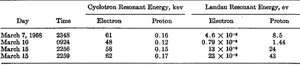
There are two possible cyclotron resonances: normal cyclotron resonance with electrons and anomalous cyclotron resonance with protons. In the first case, the right-handed wave and the electron propagate in opposite directions. The parallel velocity of the electron Doppler shifts the wave frequency so that the electron experiences a fluctuating field at its gyrofrequency. In the second case, the proton and the wave travel in the same direction. The proton travels faster than the waves and thus the proton experiences a fluctuating left-handed field. This resonance condition only specifies the parallel velocity of the resonating particle. To find this resonant velocity, we have again used cold plasma theory and the measured wave and solar wind properties for the same four events previously studied. Table 3 lists the parallel resonant energy equivalent to this velocity. These energies are about 60 keV for electrons and 0.15 keV for protons.

The resonant electrons do not fit our criteria for the source of energy for these waves, since to create a wave traveling against the solar wind these particles must be traveling with the solar wind. Our source particles should be streaming against the solar wind. Furthermore, although such electrons have been seen in the solar wind, their energy density is low. We expect, therefore, that such electrons are not the source of such waves and are a very poor sink for them.

The resonant protons do fit some of our criteria for a source, since they generate up- stream waves while themselves moving against the solar wind. Furthermore, they are moving faster than the waves. However, the velocity equivalent to energy given in Table 3 is only about 170 km/sec and is not sufficient to move upstream from the bow shock along the field lines. In other words, the cyclotron resonant protons must also be traveling toward the bow shock, although not as fast as the solar wind particles. This again, rules out a cyclotron resonance with shock generated particles as a source for such waves. Also, such particles do not appear to possess a significant fraction of the solar wind energy and at most may contribute to weak cyclotron damping. We note that this cyclotron resonance with protons moving against the solar wind is the same mechanism proposed by Barnes [1970] to create the low-frequency waves. The mechanism is successful for lower frequencies because the resonant parallel velocity of the protons is, among other things, proportional to the proton gyrofrequency divided by the wave frequency. This ratio is much greater for the waves considered by Barnes, although the wave phase velocities are comparable to those of the waves considered here. Thus, the protons in Barnes' mechanism can travel upstream.

Table 3. The possible Cyclotron and Landau Resonant Energies with Protons and Electrons for the Four Wave Packets

There are also two possible Landau resonances, one with electrons and one with protons, in which the phase velocity of the wave parallel to the field matches the velocity of the particle parallel to the field. The energies equivalent to these parallel velocities are also listed in Table 3. These energies are much smaller than for cyclotron resonance and appear even less likely to provide a source or a damping mechanism. The spread in energies is also quite large as opposed to the cyclotron resonant energies, which were remarkably constant. It appears that these possible simple wave-particle interactions provide no clear indication of the source of these wave packets.

In considering sources for these wave packets, we must also consider the amplitude envelope, which has a quite characteristic shape. There is usually a sharp spike followed by a decaying wave train. It is tempting to interpret this as the steepening of a hydromagnetic wave as was done by Heppner et al. [1967]. However, our analysis shows that the wave is being swept past the observer. In the solar wind rest frame, therefore, the spike, or amplitude maximum, is at the trailing edge of the wave packet. This at first appears to be a strange result. Such a situation however, is often found at the shock front [Heppner et al., 1967; Olson et al., 1969] where a leading wave train or precursor exists. Furthermore, Knox [1969] studied electron cyclotron resonance of finite amplitude whistler mode waves and showed that, although wave trains with leading spikes are expected in general, the spike may be at the end of the wave packet under certain conditions. Thus a study of the propagation of wave packets in the solar wind in cyclotron resonance with protons might check our interpretation of these waves.

Another interpretation of the discrete wave packets is that they do not represent free modes governed by the dispersion relation but in fact are forced modes. The slow increasing amplitude of the wave, which owing to Doppler shifting we observe as a slow decrease with time, represents the growth of the wave in the presence of a source. The rapid decrease in amplitude, which owing to Doppler shifting we observe as a rapid increase, represents the cyclotron damping after the source has passed (R. W. Fredricks, personal communication).

Thus, the waves must be generated in the solar wind plasma in the presence of reverse flow particles from the earth's bow shock. The source does not appear to be due to a cyclotron instability with either the reverse flow protons or electrons. Furthermore, neither the cyclotron resonant particles nor the Landau resonant particles are major constituents of the solar plasma. The source mechanism and possible damping mechanism remain unidentified.

SUMMARY AND CONCLUSIONS

In addition to the waves with apparent frequencies near 0.01 Hz that are found in the solar wind, in association with the intersection of the field line with the earth's bow shock, wave packets at frequencies near 0.4 Hz often exist. Since they are usually found in conjunction with the lower frequency waves, they probably are also associated with the near presence of the bow shock. In the spacecraft frame these wave packets commonly rise quickly to maximum amplitude and then decay more slowly. The peak-to-peak amplitudes typically are about 4 nT, and the waves last about 3 cycles. However, durations of 9 cycles and amplitudes of 14 nT have been recorded. Although these waves generally appear left-handed, they have the same properties as right-handed waves in a cold plasma at about twice the proton gyrofrequency. Thus, they appear to be right-handed waves propagating against the solar wind but being swept across the observer because their phase velocity is less than the solar wind velocity, and thus appear to be undergoing a polarization reversal. Estimates of the wave frequency for a limited number of cases, made by using cold plasma theory and the measured solar wind parameters, give an average frequency of about 1.2 W _p.

These waves could not propagate from the bow shock and therefore they must originate in the solar plasma, presumably because of the alteration of the distribution functions of the solar wind plasma by the presence of reverse flow particles originating at the bow shock. Cyclotron and Landau resonance, with both protons and electrons, give energies too high or low to result in important wave effects. Since these waves are well defined and occur frequently although not constantly, they should provide a good plasma diagnostic in this interaction region. It is hoped that these waves have been adequately described to enable this to be done. Further comparisons with other field experiments and particle experiments on the same spacecraft may provide more information on the possible mechanisms [Scarf et al., 1970].

ACKNOWLEDGMENTS.

We are deeply grateful to Marcia Neugebauer for providing the data from the JPL solar wind experiment. We also benefited from discussions of these results with R. L. McPherron, T. G. Northrop, J. V. Olson, and F. L. Scarf. The co-investigators responsible for the UCLA Ogo 5 fluxgate magnetometer are P. J. Coleman, Jr., T. A. Farley, and D. Judge.

This work was supported by the National Aeronautics and Space Administration under contract NAS 5-9098.

The Editor wishes to thank D. H. Fairfield and R. W. Fredricks for their assistance in evaluating this paper.

REFERENCES

(Received August 21, 1970;

revised October 15, 1970.)

Back to CT Russell's page More On-line Resources
Back to the SSC Home Page